Performance Modelling

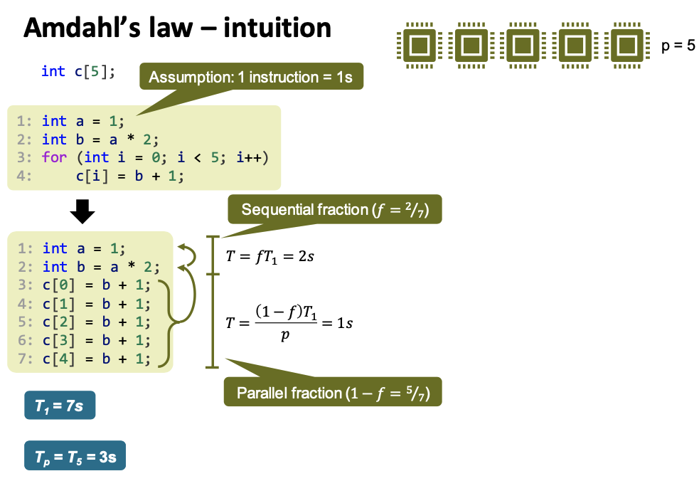
Amdahl’s law

Formally:

Amdahl’s law:

• A program runs in time $T_1$ on one processor.
• A fraction 𝑓, $0 ≤ 𝑓 ≤ 1$, of it is sequential.
• Let $T_p$ be the runtime on p processors, then \(T_p \geq fT_1 + \frac {(1-f)T_1}{p}\)

Speedup	\(S_p= \frac {T_1} {T_p} \leq \frac 1 {\frac {1-f}{p} +f}\)
Efficiency	\(S_p= \frac {S_p} {p} \leq \frac 1 { {1-f} +fp}\)

---

For $p \rightarrow \infty$,

\[T_\infty\geq fT_1\] \[S_\infty \leq \frac 1 f\] \[E_\infty = 0 \text{ if } f \neq 0\]

However, Amdahl’s law describes the best, ideal case. In reality, things look much worse. For example, even with very little sequential code $(f=0.05)$, the maximum speedup achievable with infinitely many processors is only $20$.

This is due to a number of factors, such as:

• No perfect load balancing

• Parallelization overhead $O_p$

  \[S_p = \frac {T_1} {T_p + O_p}\]
• The parallel portion is not infinitely parallelizable

Why do large-scale Clusters work?

More processors → more memory → solve larger problem size

Gustafson–Barsis’ Law

If the sequential part $𝑓$ approaches $0$ for large problem sizes $n$, then \(S_\infty (n) \leq \frac 1 {f(n) }\xrightarrow[n \rightarrow \infty]{} \infty\)

Strong vs Weak Scaling

Strong Scaling(Amdahl’s Law)	Weak Scaling (Gustafson-Barsis’ Law)
Describes behavior of $S_p(n)$ for fixed $n$ and $p → ∞$	Describes behavior of $S_p(n)$ for $n, p → ∞$
Complete the same amount of work faster	More processors allow us to do more work

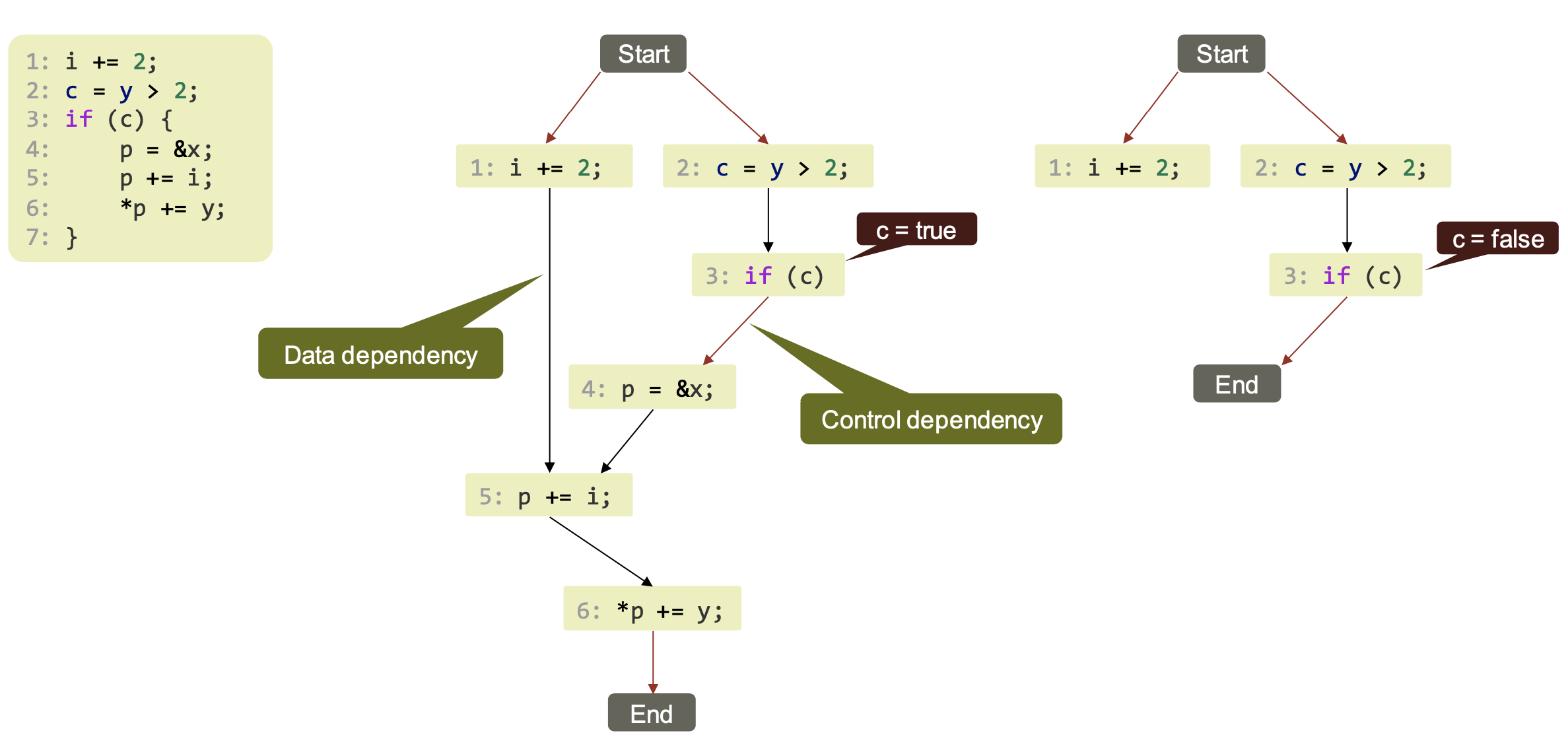
The next level of detail: execution traces

Abstract program view to reason about execution of program.

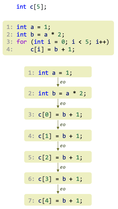
Execution Trace

Order in which program instructions are executed, given as sequence of instructions. It depends on both program code and program inputs.

• $\xrightarrow{eo}$: Execution order
• $u \xrightarrow{eo} v$: instruction $u$ completes before instruction $v$ is executed

From traces to execution DAGs

Execution order $\xrightarrow{eo}$ is a total order (implies sequential execution)

• What about parallel execution?
• What can run in parallel?
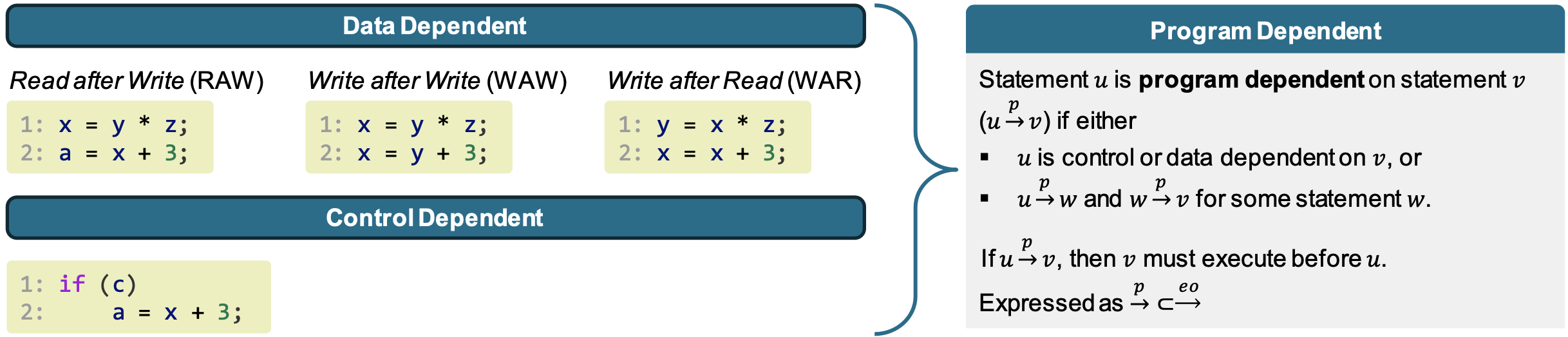
  • “independent” program statements

$\xrightarrow{p}$ forms a directed acyclic graph (DAG) of the program → Execution DAG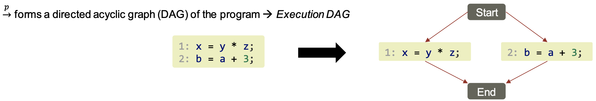

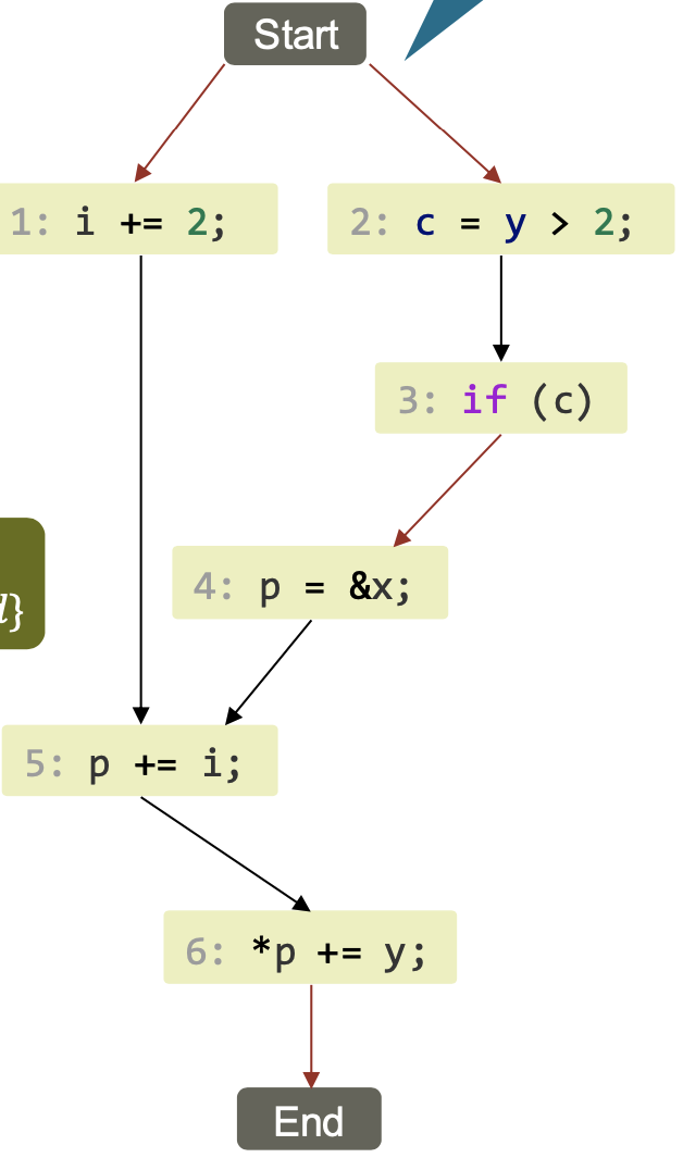
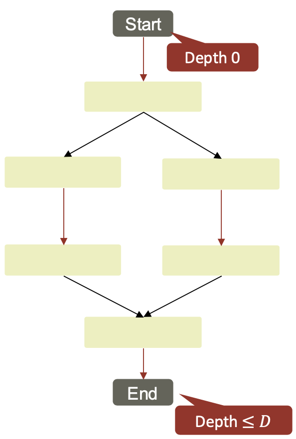
Example DAG

Work and Depth Metrics

Work: $W(n) =$ number of nodes in EDAG

Depth: $D(n) =$ number of nodes on longest path from Start to End

Average parallelism: $\frac {W(n)}{D(n)}$

Example $W = 6, = 5$	Example: Reduction $(x_0, x_1, …, x_{n-1})$

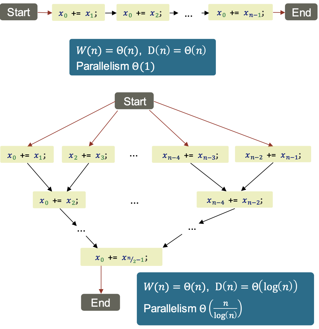Example: Mergesort

sort(L):
  if length(L)<2: return L;

  L1 = sort(left(L));
  L2 = sort(right(L));

  return merge(L1, L2);

Work	$W(n)= \theta(n\log n)$
Depth	$D(n)=D(\frac n 2) + \theta(n) = \theta(n)$
Parallelism	$\theta(\log n)$

→ Parallel merge with better $D(n)$ exists

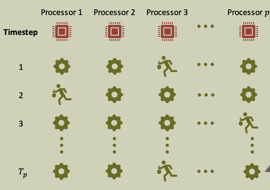
Scheduling EDAGs to Machines

Simple machine model for parallel computing (idealized shared memory multiprocessor)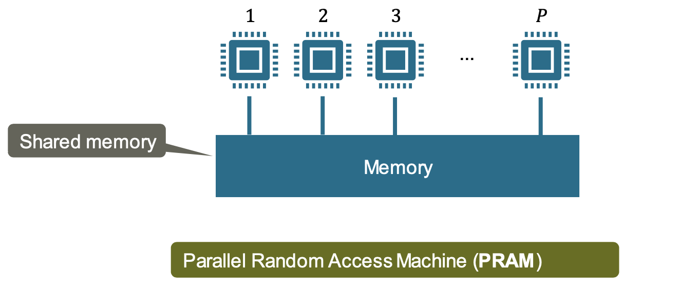

1. Instructions, including memory accesses, execute in unit time.
2. Processors progress in lockstep (each time step, each processor executes one instruction)

---

Scheduler

Function that, given EDAG, selects at most $P$ ready instructions for execution at next time step

Offline scheduler: computes schedule in advance

Online scheduler: next instructions based on past instructions and set of ready instructions

Scheduling Lower Bound (PRAM): \(T_p \geq \max (\frac W P, D)\)

Proof:

• Total number of instructions = $W ≤ P ⋅ T_P$
• Each step can execute $≤ 1$ instruction on a directed path of the EDAG → $ ≤ T_P$

Greedy Scheduler

Idea: Do as much as possible in every step

Ready node

a node is ready if all predecessors have been executed

Greedy Scheduling Procedure (Online)

Complete Step: #{ready nodes} $≥ P$

• → Run any P nodes from the set of ready nodes
• Number of complete steps $\leq \frac W P$

Incomplete Step: #{ready nodes} $< P$

• → Run all ready nodes
• Number of incomplete steps $\leq D$

Brent’s Lemma

Any greedy scheduler achieves execution time \(T_p \leq \frac {W+(P-1)D} P\)

Greedy Scheduler: Sketch

Maintain task pile of unfinished tasks, each ready or not. Initial root task in task pile with all processors idle.

Pile needs concurrency-control / locking!

At each step, processors are idle or have a task t to work on:

If idle:
 Get an (arbitrary) ready task from pile

If working on task t:
  Case 0
    t has another instruction to execute → execute it
  Case 1
    t spawns task s → return t to pile, continue with s
  Case 2
    t stalls → return t to pile and idle
  Case 3
    t dies (finishes) → continue with parent p or idle
    (if p has living children)

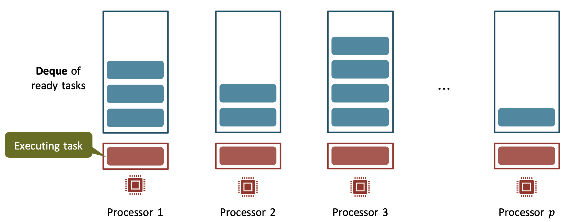
Work-stealing scheduler

The centralized workpile of the greedy scheduler can become a bottleneck when the number of processors is large.

Each processor maintains its own workpile:

• All processors do only useful work and operate locally as long as there is work
• Processors with empty work-piles will try to steal tasks

At each step, we associate with each executing or ready task a node of the EDAG.

Each vspawn operation spawns exactly two children tasks. Spawns of more than two tasks are replaced by a binary tree of operations that spawn a pair of tasks.

If a task enabled 2 children, 1 of them is pushed to the local work-pile and the other is executed next.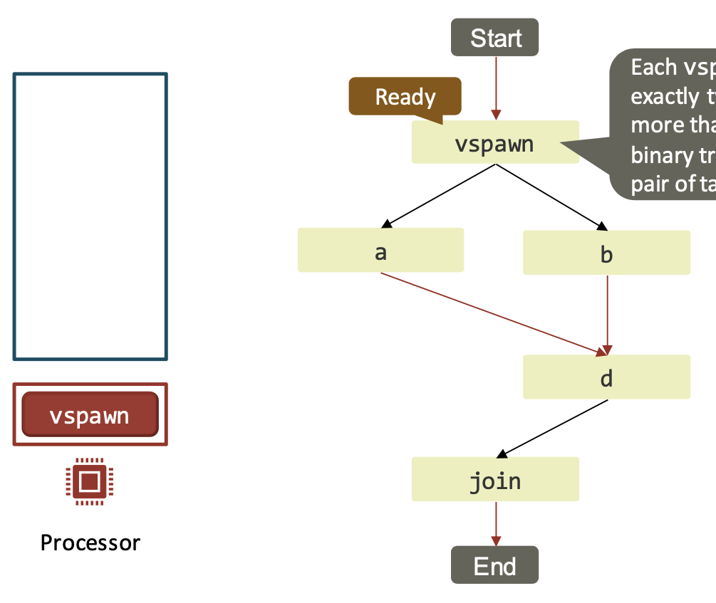
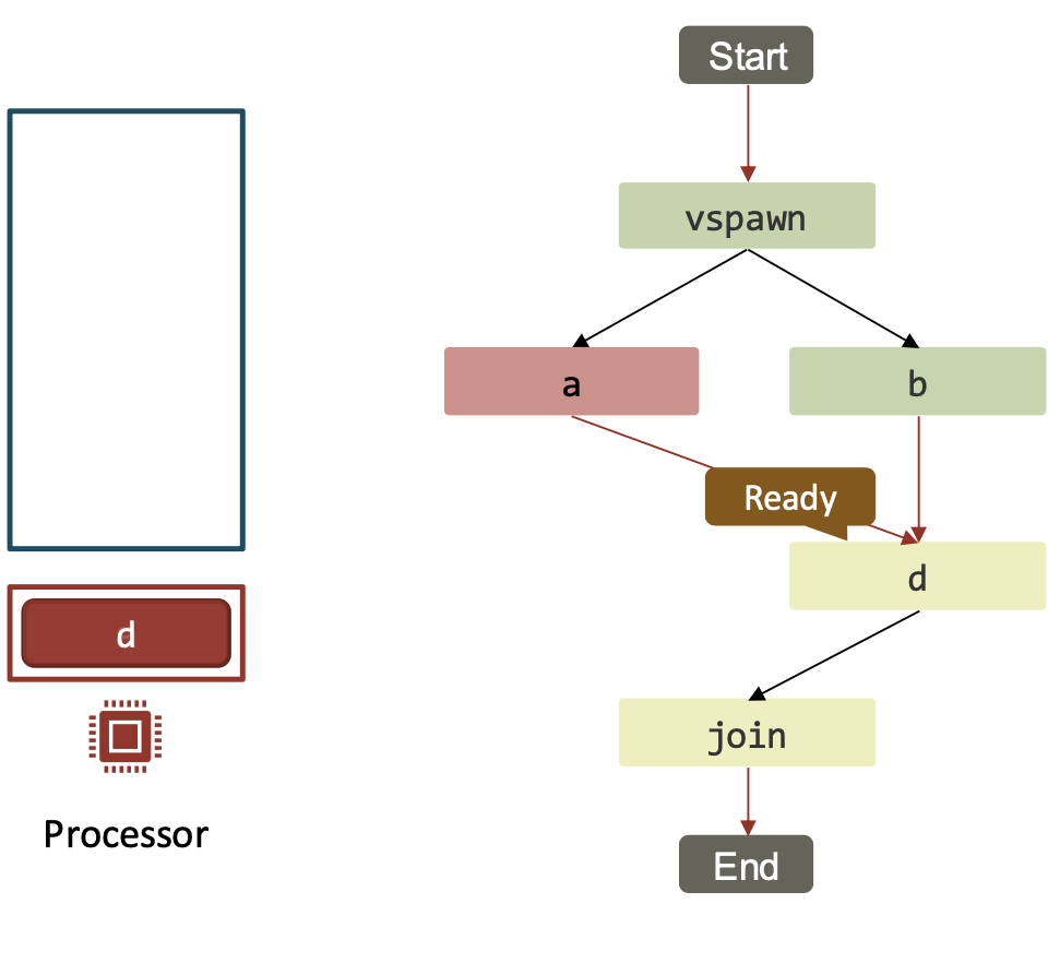
If a task enabled 1 child, it will continue executing that child.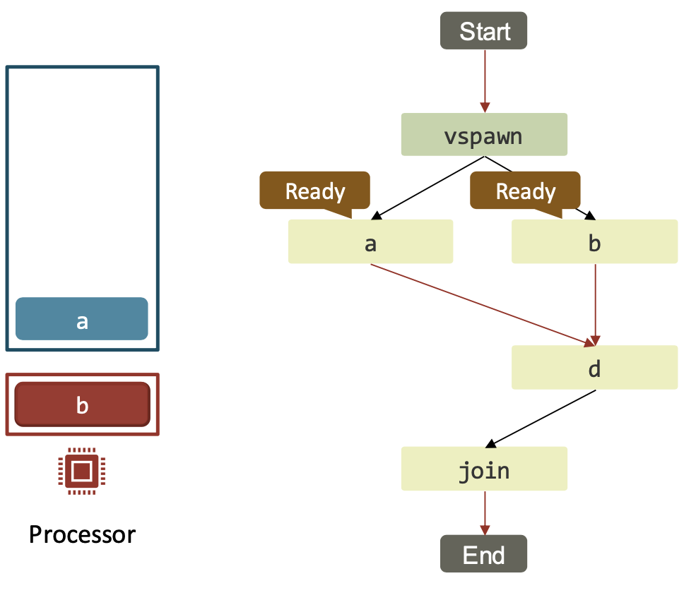

• The depth of the enabling tree is less or equal to the depth of the EDAG.
• The exact structure of the enabling tree depends on the scheduler.

Work-stealing scheduler – enabling tree example

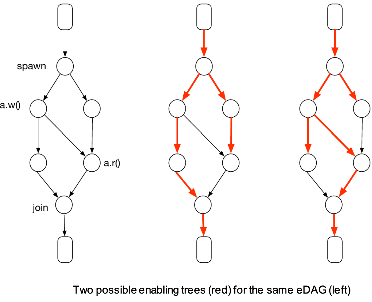
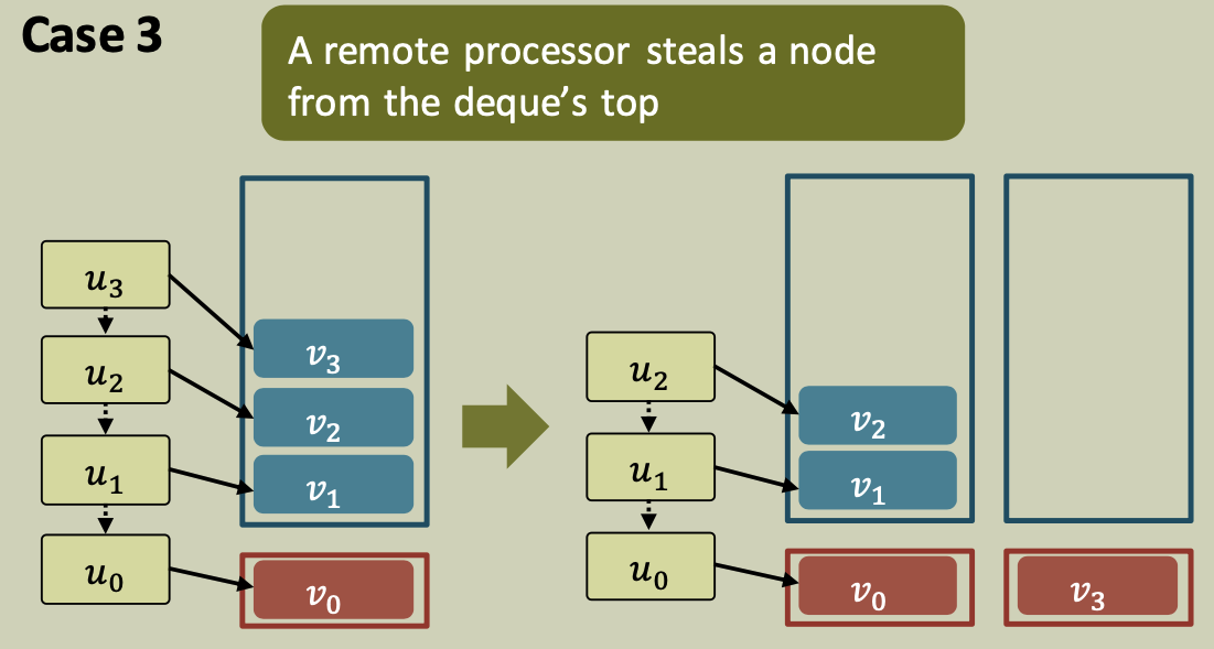
If the deque is empty, it will attempt to steal a node from the top of another randomly chosen deque.

A steal may fail if the target deque has 0 or 1 entries or was successfully targeted by another stealer.

Stealing is overhead! How do we know that we are not stealing all the time, leading to sequential performance (no speedup)?

Work stealing scheduler: Proof sketch

Lemma 1

If $S$ is the number of attempted steals then

\[T_P = \frac {W + S} P \qquad \longrightarrow \qquad P \cdot T_P = S + W\]

At each time-step, a processor either executes a task or attempts a steal.

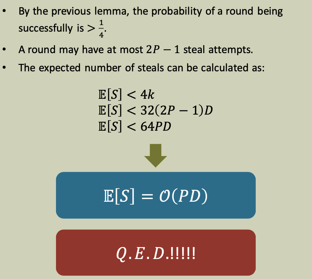
Thesis

The goal of the proof is to show that the expected number of steal attempt is

\[\mathbb{E} [S] = O(PD) \longrightarrow \mathbb{E} [T_P] = \mathbb{E} [\frac {(W+S)}P] = O(\frac W P + D)\]

---

Remember: Brent’s lemma for a greedy scheduler \(T_P \leq \frac {W+(P-1)D} P\)

The depth is an upper bound on the number of timesteps where some processor is idle (similar to Brent’s lemma), so that the total number of idling work cycles is $O(PD)$.

Lemma 2: Structural lemma

• For any of the $P$ deques, the parents of the nodes in the deque always lie on some root-to-leaf path of the enabling tree.
• The order of the parents along this path corresponds to the top-to-bottom order of the nodes in the deque.

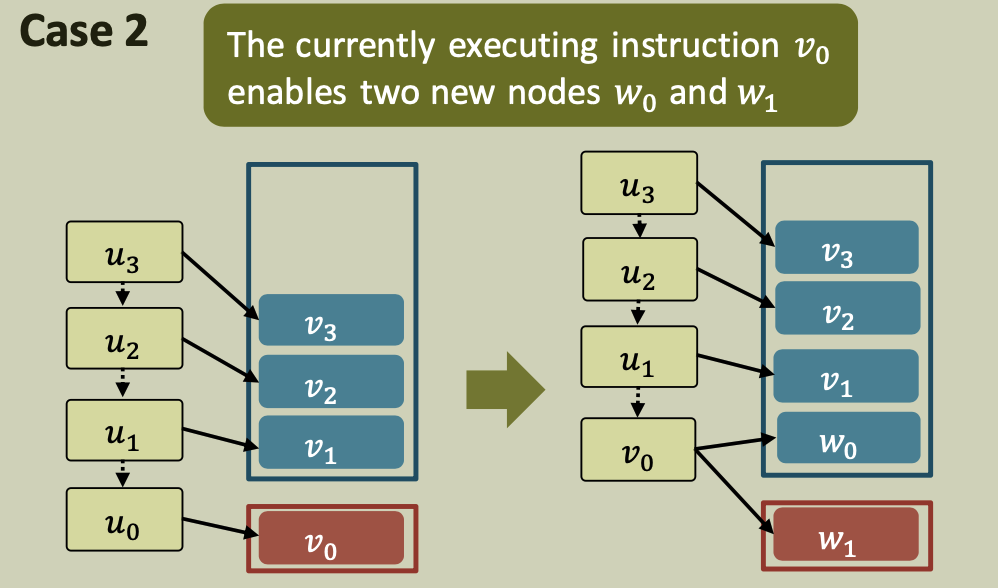
Let $v_1,…,v_k$ denote those nodes ordered from the bottom to the top. If there is an executing node on that processor, denote it as $v_0$.

Let $u_i$ be the node that enabled $v_i$. Then, $\forall \; 0 < i ≤ k$, node $u_i$ is an ancestor of node $u_{i-1}$ in the enabling tree.

While we may have $u_0$ = $u_1$, for all $i \neq 0$, $u_i \neq u_{i+1}$

No new node	$1$ new node	$2$ new nodes	Steal

Corollary 1

We define the depth $d(u)$ of a node to be the distance of node $u$ from the root (start) in the enabling tree. $\rightarrow$ Structural lemma $\rightarrow$

Corollary 1

If $v_1,…,v_k$ are nodes in a deque ordered from the bottom to the top, and $v_0$ is the currently executing node, then we have $d(v_0) ≥ d(v_1) > ⋯ > d(v_k)$.

The levels of nodes (excluding the currently executing node) in each deque are strictly increasing from top to bottom.

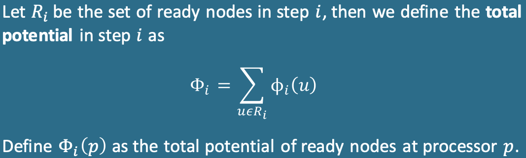
Potential function

We define a potential function $\phi_i (u)$ at step $i$ for a ready node $u$ as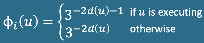

We show that the potential is monotonic and non-increasing. We show that each possible transition decreases the potential (i.e., $\phi_{i+1} \leq \phi_i$ ). The 4 cases are the same as those from the structural lemma.

Note that a failed steal does not change the potential.

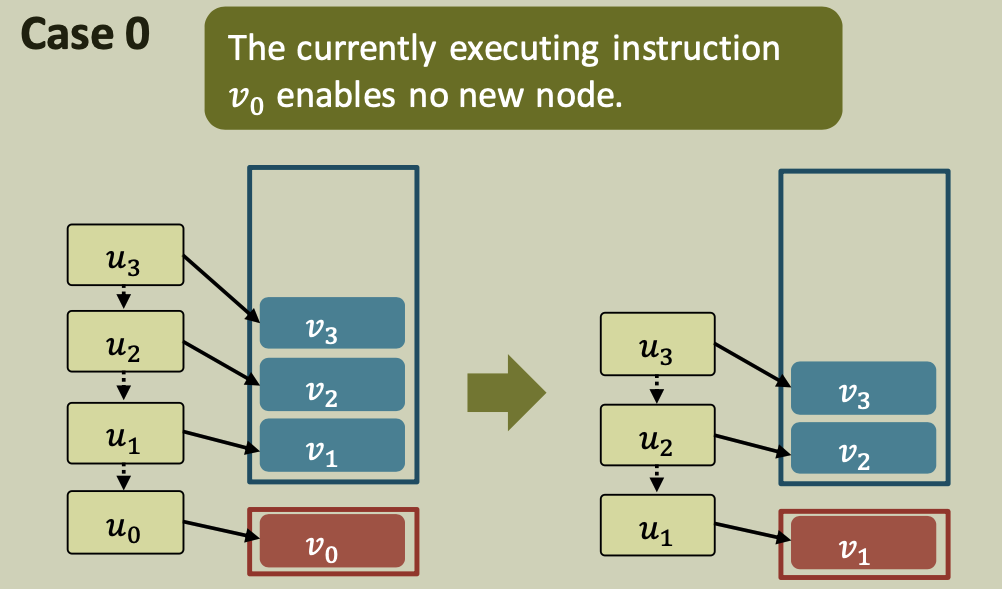
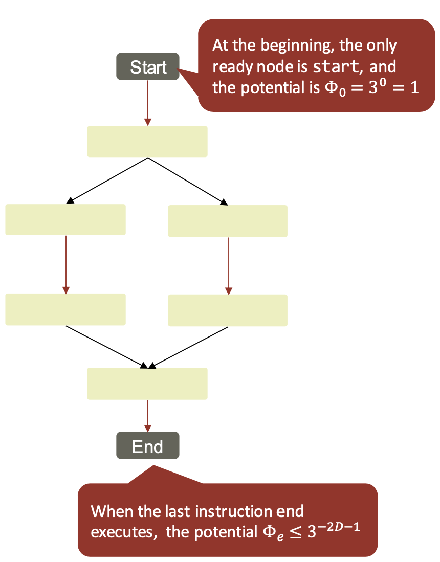
Case 0

A processor finishes the execution of a node u that enables no new node.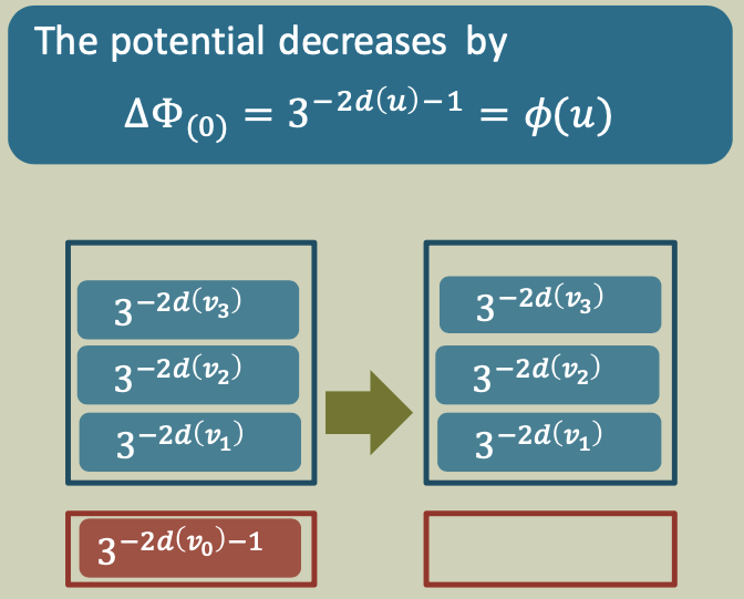

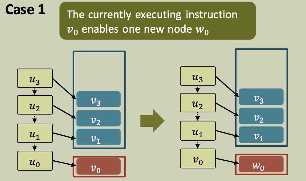
Case 1

A processor finishes the execution of a node $u$ that enables a new node $v$ to be executed immediately. Node $v$ is the child of $u$ in the enabling tree so that \(d(v)=d(u)+1\)

Case 2

A processor finishes the execution of a node $u$ that enables 2 new nodes $v$ and $w$, one being executed. Without loss of generality, assume that $v$ is executed and $w$ is pushed to the lower end of the deque.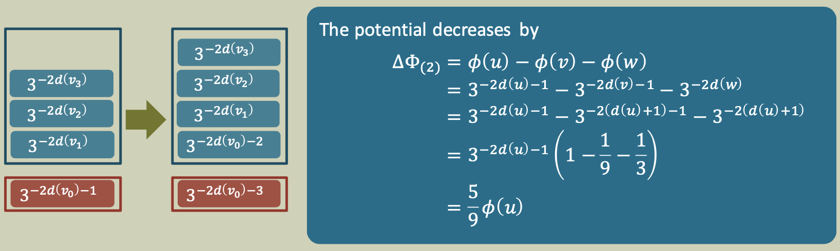

Case 3

A processor steals a node $u$ from the top of some other deque and readies it for execution.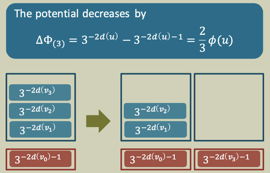

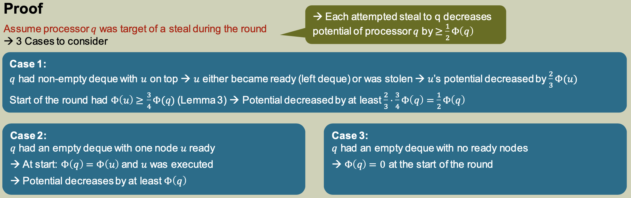
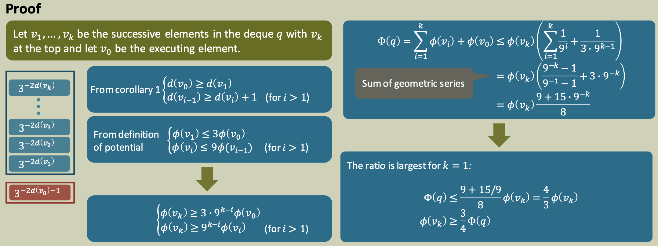
Lemma 3: Top-heavy Deques

The top element in any non-empty deque has at least $\frac 3 4$ of the total potential of the deque.

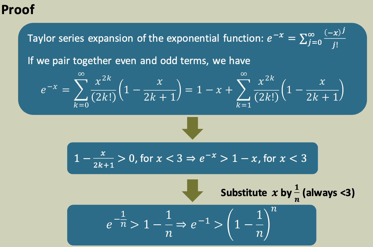
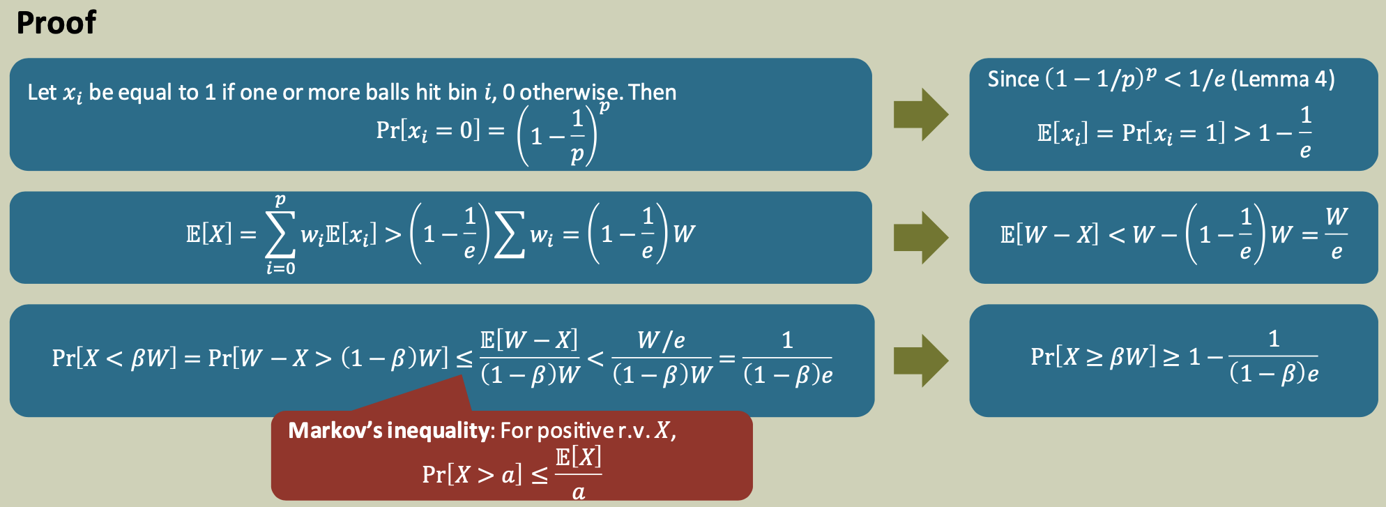
Lemma 4

For $n>1$, \((1-\frac 1 n)^n<\frac 1 e\)

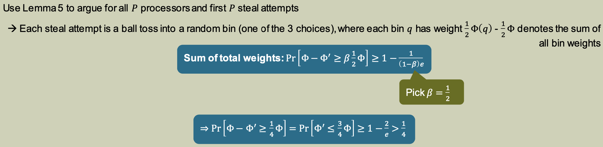
Lemma 5: Balls and weighted bins

Consider the following game: $p$ balls are tossed into $p$ bins. Each bin $i$ is associated with a weight $𝑤_i$ . Assume that the balls are equally likely to hit each bin, and all tosses are independent. What is the total weight of the non-empty bins?

Lemma 5

Let $W=\sum w_i$ and let 𝑋 be the total weight of the non-empty bins. Then for any $0 < \beta < 1$, \(Pr[X\geq \beta W] \geq 1- \frac 1 {(1-\beta)e}\)

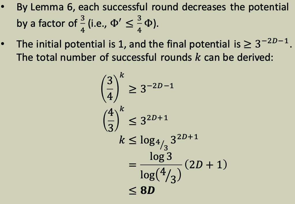
Lemma 6

One step before the end of the round, we have at most $P-1$ steals and in the last step of the round, we can add at most $P$ steals, thus a round may have between $P$ and $2P-1$ steal attempts.

We first show that a round decreases the potential by a fixed fraction with high probability.

---

Lemma 6

Let $\Phi$ be the potential at the start of a round and let $\Phi’$ be the potential at the end of the round. Then \(Pr[(\Phi - \Phi') \geq \frac 1 4 \phi] > \frac 1 4\)