Congestion Control

Assumption	We can find the optimal sending rate over several RTTs.
Doubt	In the modern internet, we often send only small requests.
Question	Do we even have enough time to ramp up?

Oscillations in TCP occur over the course of many RTTs. How big do our requests need to be for that to be realistic? On a 1Gbit/s link with 10ms RTT, we could send up to 1.25MB in a single RTT.

Study of a campus network in 2021 90% of flows are smaller than 1 kB.

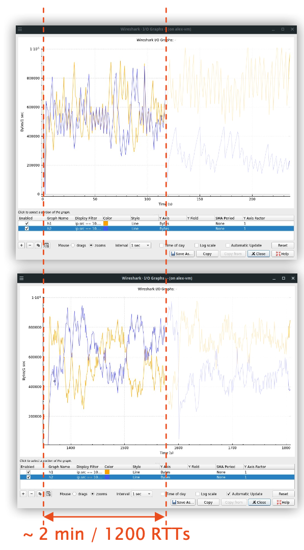
Assumption	Fairness is guaranteed on average for long running flows.
Doubt	In the modern internet, we send many small requests.
Question	Do we even have enough time to be fair? Often, we don’t!

---

Congestion Control Design

Observations are intrinsically linked to our model of the network. The model also determines our actions, but more on that later.

Observations let us estimate the model state.

not observable → difficult to model without making assumptions

not modelled → no point in observing

The TCP network model is simple and consists of 3 states. We observe packet loss via duplicate ACKs and timeouts.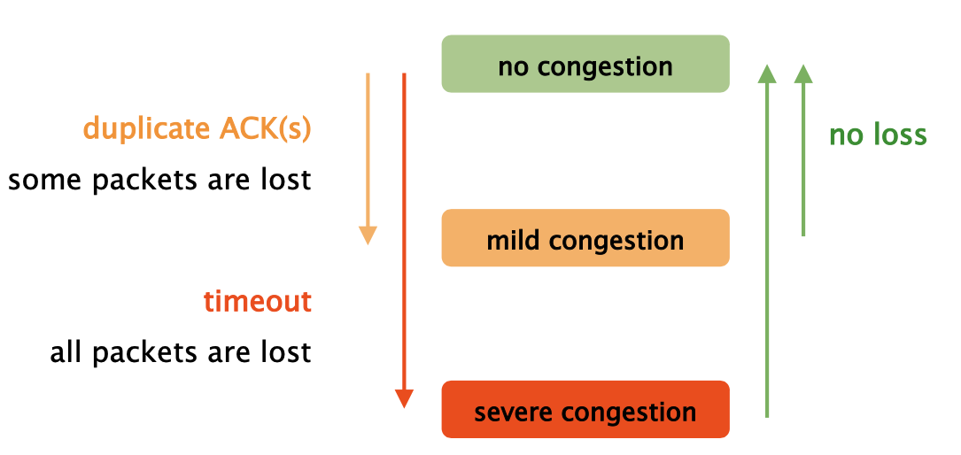
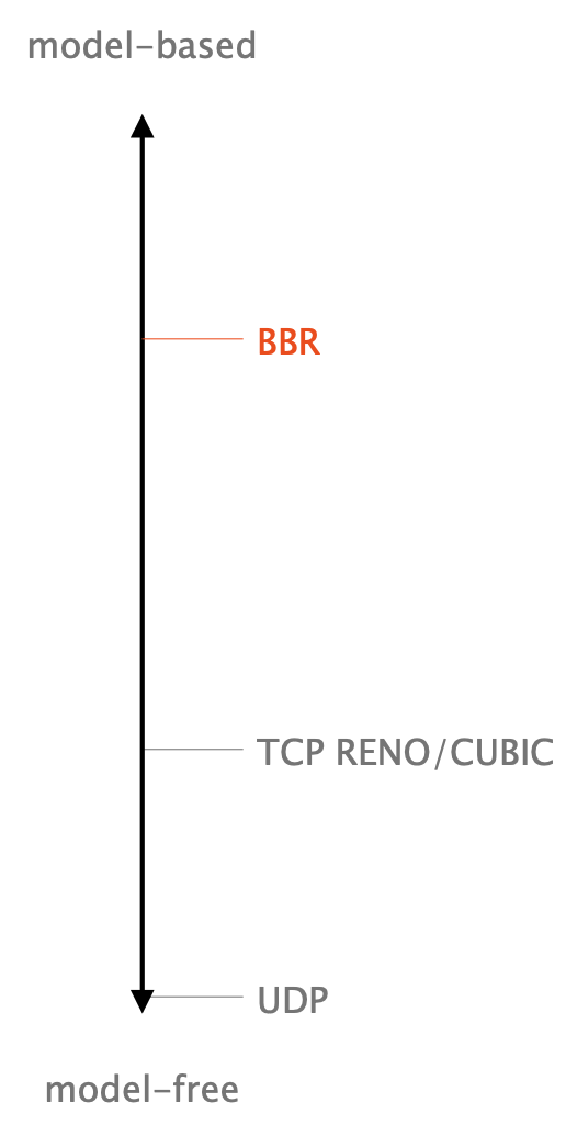
TCP RENO/CUBIC are relatively model-free algorithms: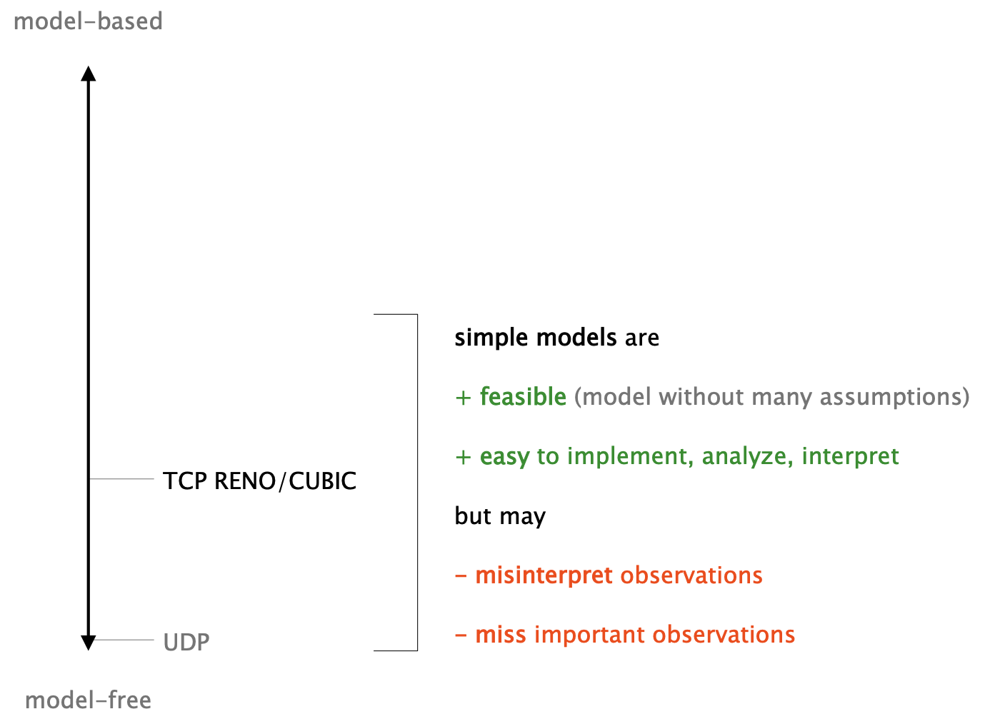
TCP RENO and CUBIC misinterpret signals: all loss is attributed to congestion, even if it is just random.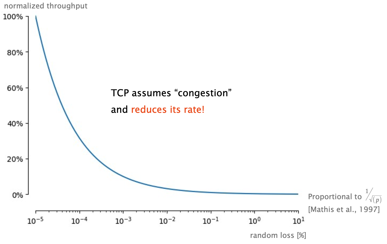
TCP RENO and CUBIC miss signals: What about delay?	Only full queues drop packets (mostly) $\rightarrow$ TCP needs to fill queues to work!

We have a two-fold problem:

1. A full queue delays congestion signals.
2. A full queue increases RTT.

Rule of thumb around 2000: buffer 250ms of incoming traffic.

Packets spend 2.5s in the buffer!

This is a problem for

• existing flows, as losses take a long time to detect, and
• new flows, as they will struggle to ramp up.
• many applications that need low latency, e.g., VoIP

This problem even got it’s own name: Bufferbloat

Where do we improve congestion control?

In the Internet?

• Limit queue size
• Active Queue Management (AQM)
  • RED: Random Early Dropping
  • CoDel: Controlled Delay

Challenges:

• Network becomes tied to the transport.
  • No separation of concerns!
• In-network drops are suboptimal.
  • Transport needs to detect it first.
• Significant overhead.
  • More computation, storage, etc.

Fundamentally, there are three things to observe:

1. Packet loss
   • observable
   • easy to model
   • when we get the signal, it’s already “too late”
2. Packet delay
   • observable, but noisy
   • difficult to model, as there are many possible causes for delay (network? receiver? …)
3. Packets in-flight
   • not fully observable,
   • difficult to model, we only know our own packets. What are other applications going to send?

On your device?

• Additional observations
• More complex models

Challenges:

• Not everything of interest is (easily) observable
• The Internet is hard to model

Should we combine both?

The network and congestion control algorithms can cooperate.

1. Provide signals in the network
2. Adjust behavior on your device

Challenges:

• Requires coordination!
• Almost exclusively used in data centres.

Explicit Congestion Notification (ECN):

• The network sets an ECN flag in the IP header when queues are getting close to full (configurable threshold)
• Last 2 bits in the “traffic class” IP header field.
• Congestion control treats ECN like a packet loss, but before any packet actually got dropped!
• Used by Data Center TCP (DCTCP)
• Network uses P4 to measure and share in-flight packets, link rate, and queue length with congestion control algorithms.
• The algorithms estimate the available bandwidth and set the optimal sending rate.
• All switches and clients must use HPCC!

Summary:

just loss as congestion signal isn’t great, but the alternatives are no silver bullets.

Control Space

A congestion control algorithm needs to decide when to send the next packet to optimize rate and/or latency.

Rate:

• how much data do we transmit successfully?

Latency:

• how quickly do individual packets arrive?

• Easy to implement.
• We mostly only need to act after an ACK has arrived.
• Update cwnd, send new packet if free space.
• Aside from that, we need coarse-grained timeouts.
• Default timeout is 200ms, does not need precise clocks!

The cwnd causes TCP connections to consist of micro-bursts.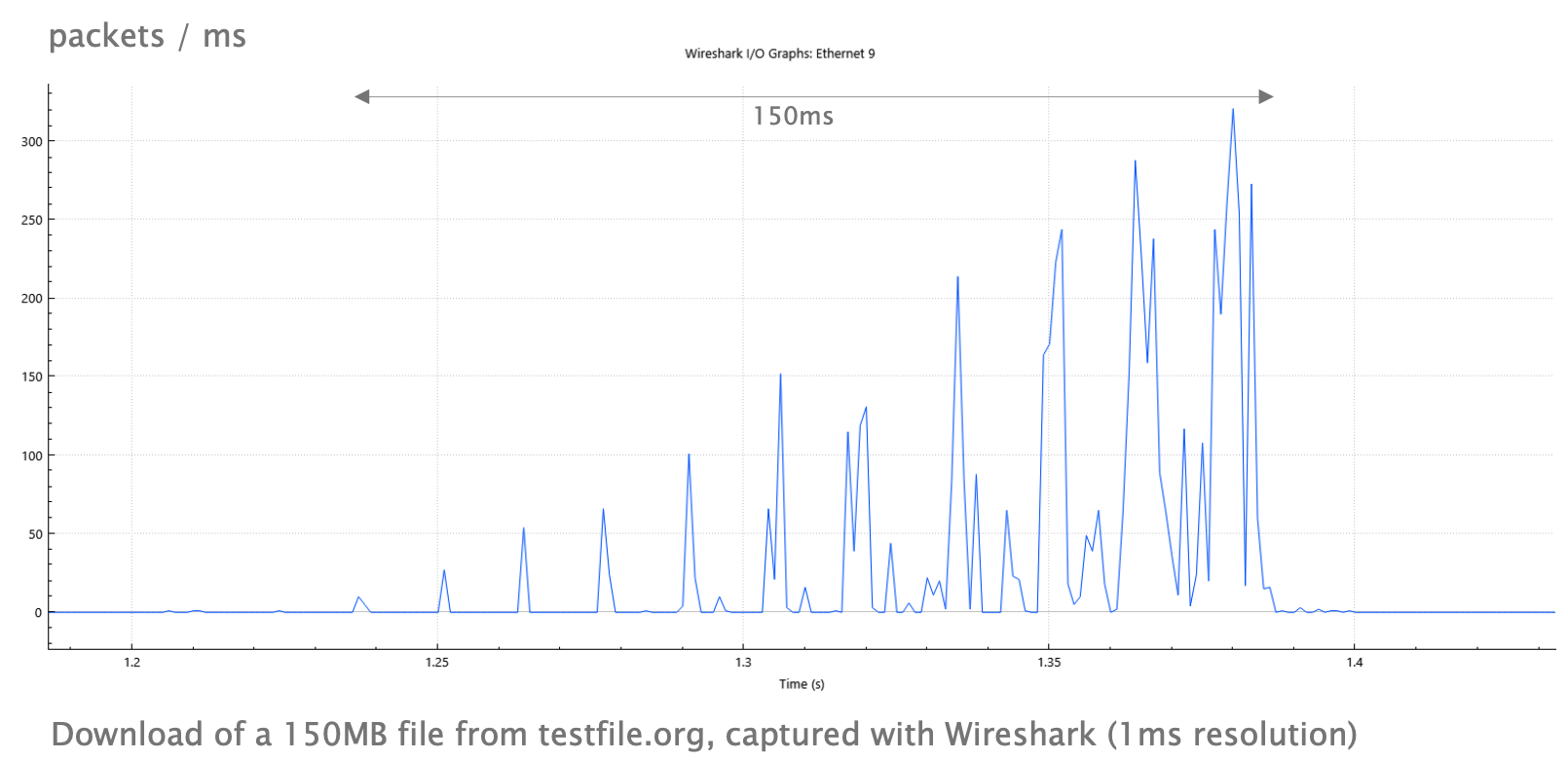

If multiple bursts coincide, we may overload queues!

Instead of sending cwnd-sized bursts, we can use pacing. The pacing rate determines the time between packets:

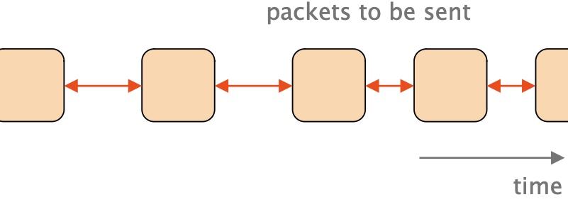
• Results in smooth traffic, at the cost of computational overhead.
  • Up to 10% of networking CPU cycles!
• Requires precise timers (or hardware support), which is not a big issue nowadays

Bottleneck Bandwidth and Round-trip propagation time (BBR)

BBR is a congestion control algorithm developed by Google in 2016.

• Available for both TCP and QUIC.
• Current version (2023): BBRv3
• BBR builds a model of the network.
• BBR is a great example for different observation and control, as we’ll discuss in the following.

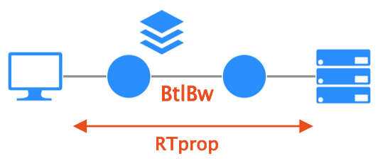
As the name implies, BBR models the network by considering the RTT and bottleneck bandwidth.

The model:

• BtlBw is the bottleneck bandwidth, i.e., the minimum rate on the path, and RTprop is the RTT.
• It does not matter how many links come before or after the bottleneck, as they faster by definition.

Why do we measure those two values? Let’s have a look at our optimization goal.

BRR controls both a congestion window and a pacing rate to maximize bandwidth while minimizing latency and losses.

• Pace packets to match BtlBw
  • Optimal rate supported by the bottleneck.
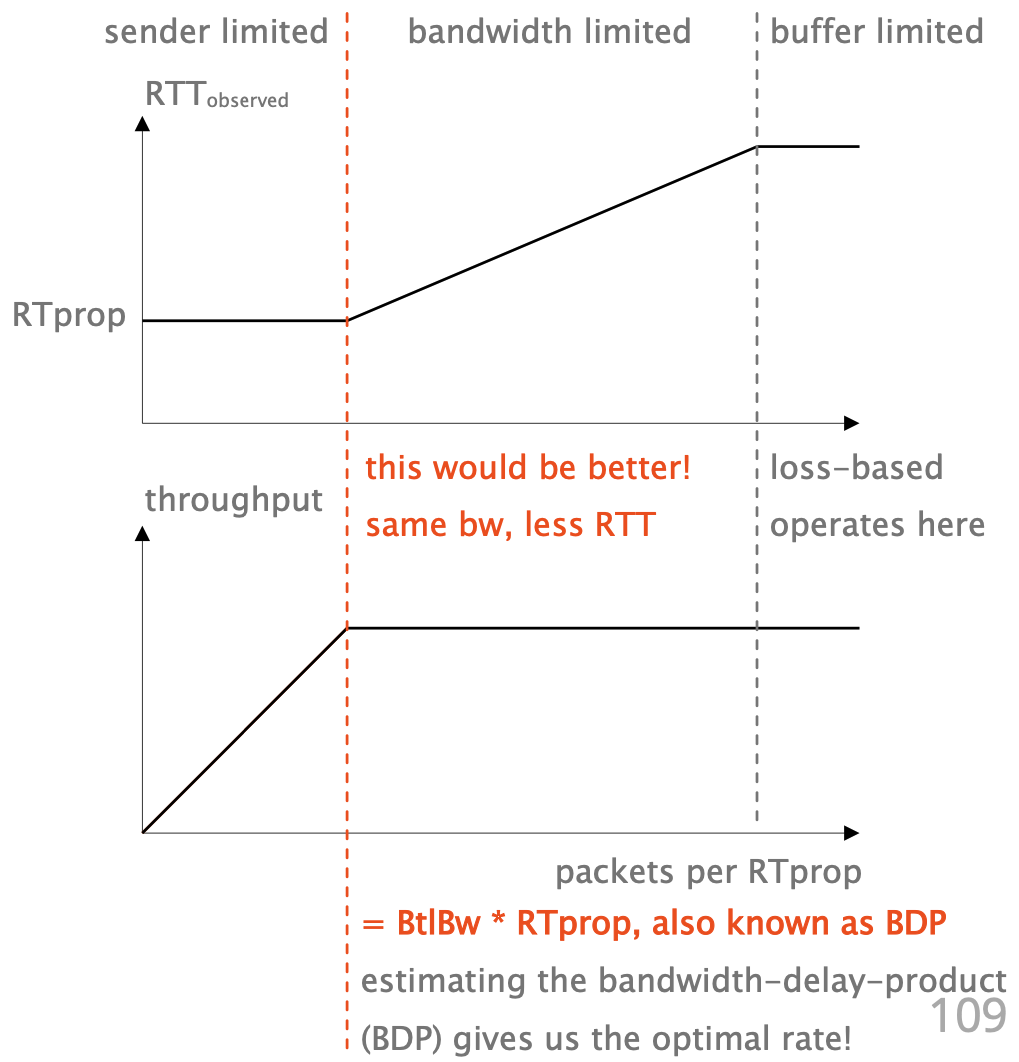
• Send until the bytes in-flight are BtlBw * RTprop
  • Less would mean that the queue runs dry.
  • More would mean that a queue builds up.
  • Sub-optimal utilization in both cases!
• We need both!
  • Pacing alone only ensures that the queue does not change, but there may be a standing queue that cannot drain.
  • The congestion window ensures that the queue can drain,
    • e.g. if BtlBw decreases we need to stop sending for a bit.

There’s a small issue. What happens if we do not send enough?

• To discover the bottleneck rate, you must exceed it!
  • But that goes against everything we want to achieve.
• Periodically (e.g. 1 of of 10 RTTs),
  • BBR probes for a higher BtlBw
• Afterwards, it reduces its pacing for a second RTT to compensate for the overhead.

Summary

BBR is an algorithm that models the bottleneck queue, measuring RTT and bandwidth, controlling pacing and cwnd.

• BBR models the queue beyond “drop → queue full” like RENO and CUBIC.
• This allows to maximize throughput at the same time as minimizing latency and loss.
• It is widely deployed at Google, and they report significant reduction in retransmissions (12%), resulting in a slight improvement in latency (0.2%).
  • 12% fewer retransmissions means 12% more network capacity for “real” traffic!

Application Layer

Applications on the Internet have many different needs. A one-size-fits-all transport cannot be optimal.

Compare a download that only needs throughput with a VoIP call that mostly cares about latency! Some applications build their own control logic on top of congestion control.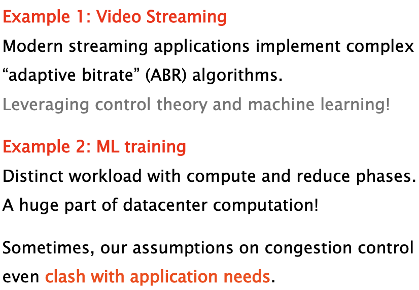

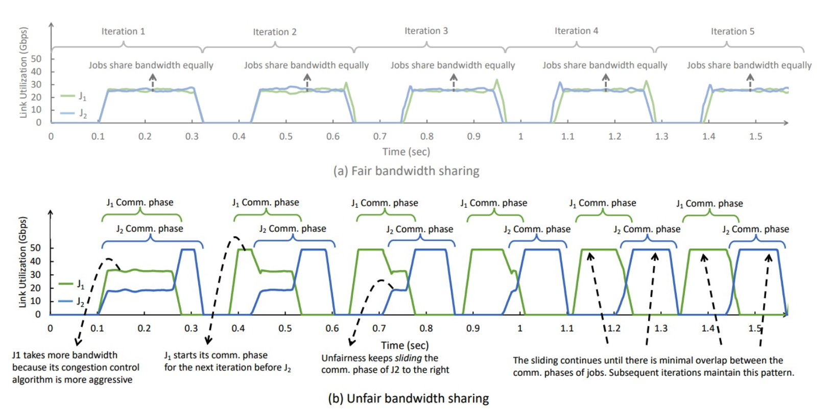
1. Assumption: Multiple flows should share bandwidth fairly.
2. Doubt: Sending data is only part of an application’s work.
3. Question: Does fair bandwidth sharing imply fair completion times?
   • Not necessarily!

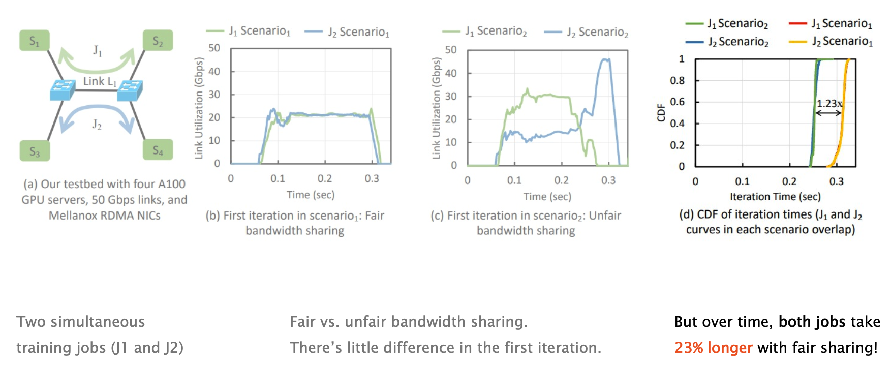
What’s going on? Many applications not only communicate, but also wait/compute.

A bit of unfairness can help to un-synchronize them.