Inference

Relationship inference

Gao-Rexford model	An abstract view of Internet routing, to formally define relationships and their export policies
Patterns in paths	Enumeration of possible GR-compliant path segments, to express paths as an array of structured elements
A heuristic algorithm	Relationship inference based on observed paths, to assemble various patterns into coherent paths

Business contracts define the pricing of the traffic exchange, thereby, the relationships between ASes.

• Customer-provider relationship
  • The customer pays its provider for access to the rest of the Internet
• Peer-to-peer relationship
  • The two peers find it mutually advantageous to exchange traffic between their respective customers;
  • typically, peers exchange a roughly even amount of traffic free of charge
• Sibling-to-sibling relationship
  • The two siblings under common ownership or control exchange traffic between their respective customers, providers, and peers without the exchange of payment

Customer-provider relationship translates into the following export policy rules:

In exchanging routing information with a provider, an AS can export its routes and its customer routes, but usually does not export its provider or peer routes.

Provider-customer relationship translates into the following export policy rules:

In exchanging routing information with a customer an AS can export its routes and its customer routes, as well as its provider and peer routes.

Peer-to-peer relationship translates into the following export policy rules:

In exchanging routing information with a peer, an AS can export its routes and its customer routes, but usually does not export its provider or peer routes

Sibling-to-sibling relationship translates into the following export policy rules:

In exchanging routing information with a sibling, an AS can export its routes and routes of its customers, and as well as its provider or peer routes

With that, we can formally define the transit property

Transit Property

AS $u$ transits traffic for AS $v$ if and only if AS $u$ transits some of its provider or peer routes to AS $v$.

• AS $u$ is a provider of AS $v$ iff $u$ transits traffic for $v$ and $v$ does not transit traffic for $u$
• AS $u$ and $v$ have a peering relationship iff neither $u$ transits traffic for $v$ nor $v$ transits traffic for $u$
• AS $u$ and $v$ have a sibling relationship iff both $u$ transits traffic for $v$ and $v$ transits traffic for $u$

Gao-Rexford guidelines provide us with an important notion: valley-free paths

Valley-free paths

After traversing a provider-to-customer or peer-to-peer edge, the AS path can not traverse a customer-to-provider or peer-to-peer edge.

a.k.a.: after you go down, you can’t go up or stay at the same level; you can only keep going down

If all ASes set their export policies according to the selective export rule, then the AS path in any BGP routing table entry is valley-free.

Formally, an AS path is valley-free if and only if the following conditions hold true:

1. A provider-to-customer edge can be followed by only provider-to-customer or sibling-to-sibling edges
2. A peer-to-peer edge can be followed by only customer-to-provider or sibling-to-sibling edges

The valley-free property enables us to identify patterns in observable AS-PATHs.

Downhill and uphill paths

Downhill path:

A sequence of edges that are either provider-to-customer or sibling-to-sibling edges

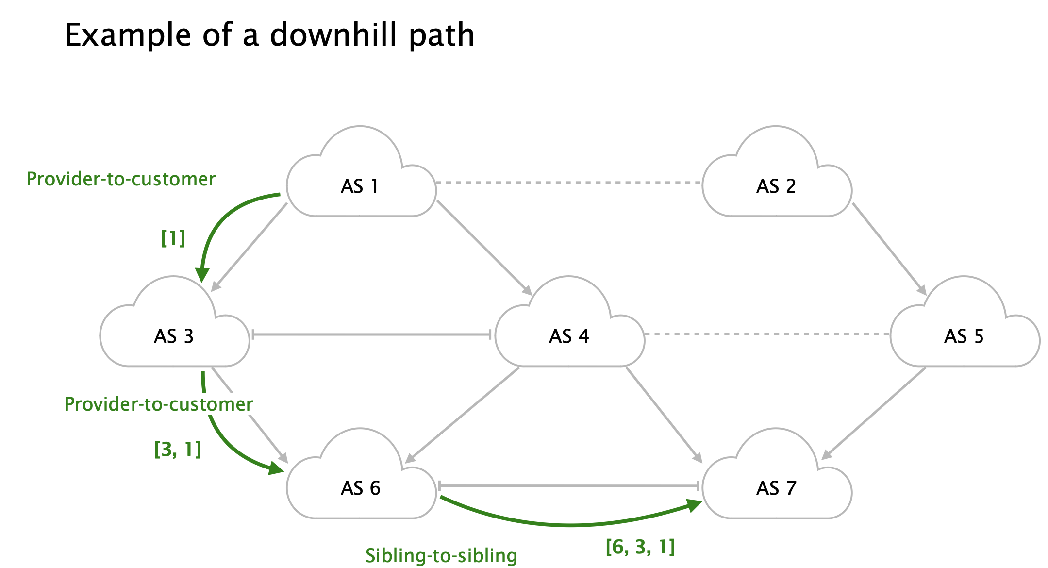
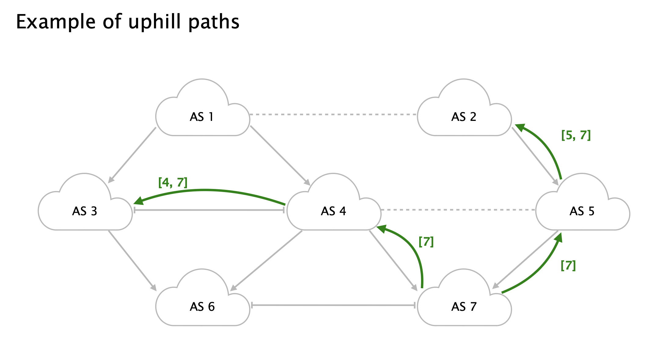
Uphill path:

A sequence of edges that are either customer-to-provider or sibling-to-sibling edges

An AS path of a BGP routing table entry has one of the following patterns:

1. an uphill path
2. a downhill path
3. an uphill path followed by a downhill path
4. an uphill path followed by a peer-to-peer edge
5. a peer-to-peer edge followed by a downhill path
6. an uphill path followed by a peer-to-peer edge, which is followed by a downhill path

This implies that an AS path can be partitioned into either

• The uphill path, the peer-to-peer edge, and the downhill path in order
• The uphill path and the downhill path in order

Top providers are the most powerful ASes within the uphill (or downhill) path in which they appear.

• The uphill top provider is the last AS in the uphill path in which it appears.
• The downhill top provider is the first AS in the downhill path in which it appears

Metrics

We need a metric to act as a proxy for business power. For this we make two assumptions:

1. AS business power: a provider typically has a larger geographical size than its customer does
2. The power metric: the geographical size of an AS is typically proportional to its degree in the AS graph

This metric leads to the following chain of reasoning:

Given

• the uphill (or downhill) top provider of an AS path should be the AS that has the highest degree among all ASes in its uphill (or downhill) path and that
• The top provider of an AS path is the AS that has a higher degree between the uphill and downhill top provider
• The top provider of an AS path is the AS that has the highest degree among all ASes in the AS path

Algorithm for inferring provider-customer and sibling relationships

• Input: BGP routing tables
• Output: Annotated AS graph G

Phase 1: Compute the degree for each AS

For each as_path(u1, u2, ..., un) in routing tables,
    For each i = 1, ..., n - 1,
        neighbor[ui] = neighbor[ui] ∪ {ui+1}
        neighbor[ui+1] = neighbor[ui+1] ∪ {ui}

For each AS u,
    degree[u] = |neighbor[u]|

neighbor[ui]

• The set of neighbor ASes for ui

⎮neighbor[ui]|

• The degree or number of neighbors for ui

---

Phase 2: Parse AS path to initialize consecutive AS pair’s transit relationship

For each as_path(u1, u2, ..., un) in routing tables,
    find the smallest j such that degree[uj] = max1 ≤ i ≤ n degree[ui]
for i = 1, ..., j - 1,
    transit[ui, ui+1] = 1
for i = j, ..., n - 1,
    transit[ui+1, ui] = 1

Transit flag for the directed edge

• An indication that the edge has been traversed as transit in the given direction

---

Phase 3: Assign relationships to AS pairs

For each as_path(u1, u2, ..., un) in routing tables,
  for i = 1, ..., n - 1,
    if transit[ui, ui+1] = 1 and transit[ui+1, ui] = 1
      edge[ui, ui+1] = sibling-to-sibling
    else if transit[ui+1, ui] = 1
      edge[ui, ui+1] = provider-to-customer
    else if transit[ui, ui+1] = 1
      edge[ui, ui+1] = customer-to-provider

Sibling-to-sibling

• An edge flagged with transit for both directions.

Customer-to-provider

• An edge flagged with transit for a single direction.

Algorithm for inferring peering relationships

• Input: BGP routing tables
• Output: Annotated AS graph G

1. Use the initial algorithm to coarsely classify AS pairs into provider-customer or sibling relationships
   • Find not peering edges
2. Identify AS pairs that cannot have a peering relationship
   • Smaller degree edge is also not peering (40 > 10) as we can not have two consecutive peer-to-peer edges
3. Assign peering relationships to AS pairs
   • Ultimately, if the degrees of two neighboring ASes are within a certain ratio (R), and no path provides a counter-example for their non-peering, we deem that relationship peer-to-peer

Localize performance issues to specific links

Some links in the Internet are sometimes lossy: their loss rate exceeds some given threshold

End-user traffic flows along paths: a path is a sequence of links between a pair of end-users

During a time interval, a path is “lossy” iff it has $≥1$ “lossy links”. All other paths are “non-lossy”.

Upon experiencing poor path performance, how can end-users locate which links are the culprit? Network performance tomography infers link performance from the network topology and path performance.

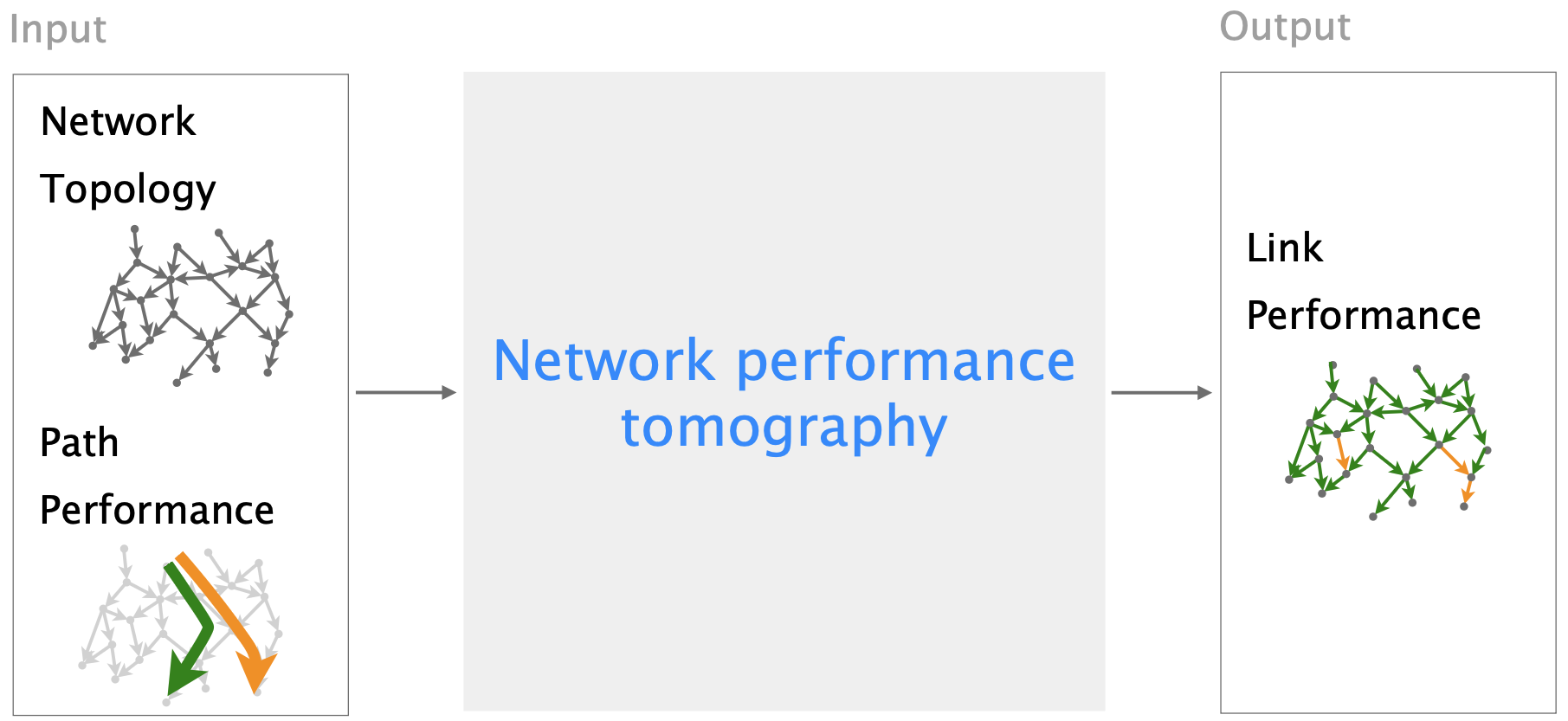
We will focus on inferring two link performance properties:

1. Probability of a link being non-lossy
2. Link Neutrality

Neutral Link

A link is neutral iff it treats “the same” traffic on different paths. Here, “the same” refers to the probability of the link being non-lossy.

Example

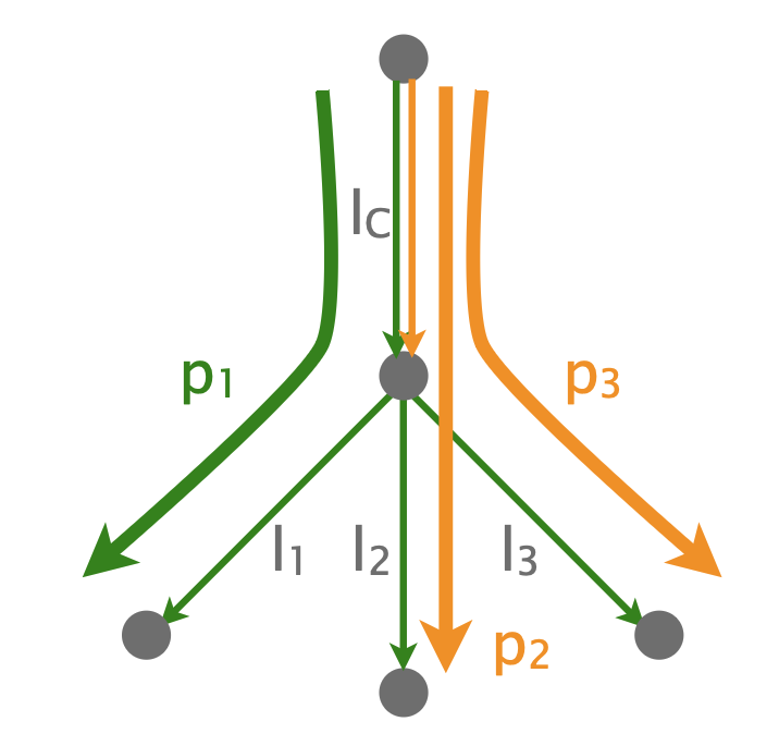
Consider a simple topology, with $3$ end-users, $1$ switch/router in the middle, $3$ links, and $2$ paths.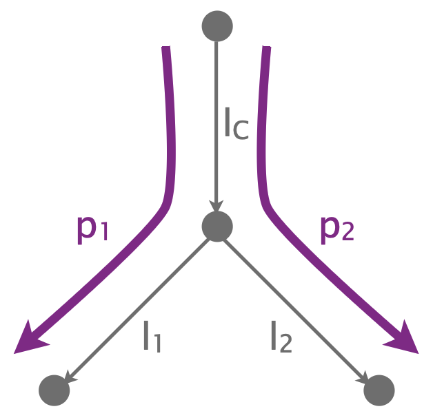

During a time interval, a link is non-lossy iff its loss rate is $<1\%$, i.e., the link delivers $≥99\%$ of the packets that arrive at this link to the next link.

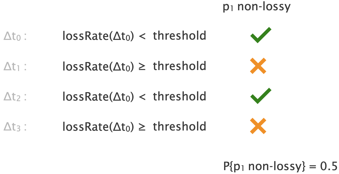
Assume that all links are always non-lossy except $l_C$, which is lossy (loss rate $≥1%$) with probability (w.p.) $0.5$

Inference

How do we infer for each link the probability of being non-lossy from the network topology and path measurements? The key idea is to relate the knowns (path performance) to the unknowns (link performance) through a system of equations.

1. We estimate the path performance, which is the probability of the path being non-lossy
   1. During a time interval, we measure the path loss rate the path is “non-lossy” iff “loss rate < threshold”
   2. ideally, we must set the threshold so that the path is non-lossy iff all its links are non-lossy
   3. In practice, we can set the threshold to only guarantee that “if the path is lossy, ≥ 1 of its links is lossy”
   4. To achieve that, we set the threshold to the maximum loss rate that the path would experience if all of its links were non-lossy
2. We measure the path performance, which is the probability of the path being non-lossy
   1. Estimate it as the fraction of time intervals during which the path is non-lossy
   2. We send S packets over p1, split the measurement time into intervals, and check for what fraction of them the path is non-lossy
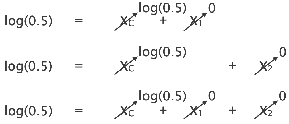
3. We build a system of equations which connects path performance to the performance of its links
   1. Here is the equation we can write for p1:
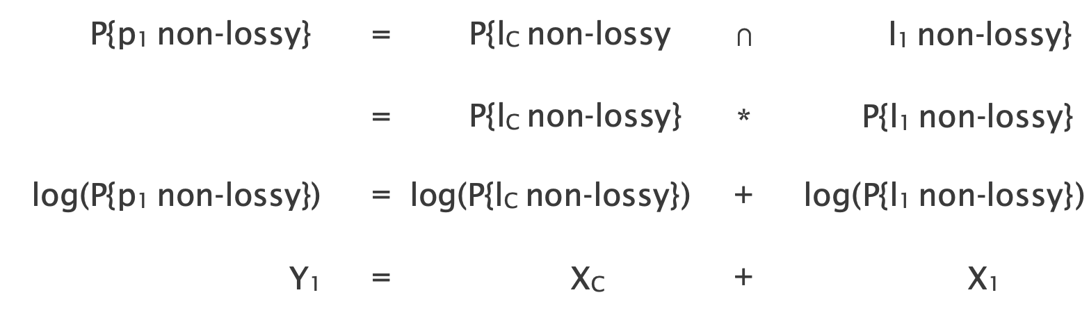
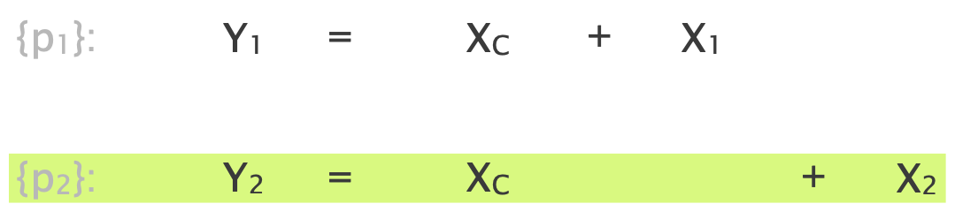
   2. And here is the equation for p2:
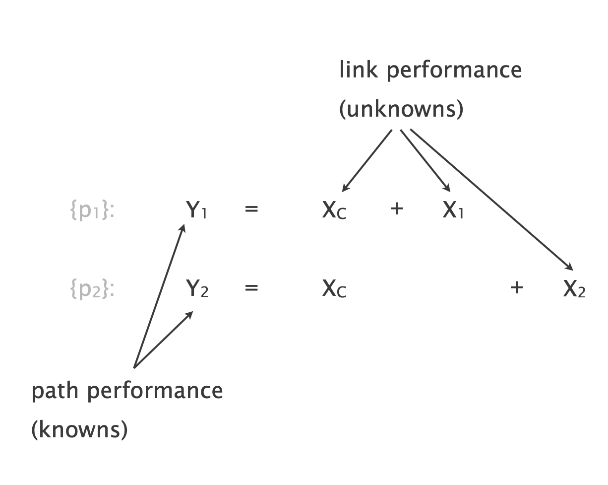
4. We solve the system of equations using linear algebra
   1. Not full-rank: only 2 equations for 3 unknowns, so multiple solutions and picking a realistic one may not be easy
   2. Considering only the performance of individual paths is not enough to create a full-rank system of equations

We need more information to further constrain the system’s

Solution: use the performance correlation among multiple paths

So far, we haven’t used how often both p1 and p2 are non-loss.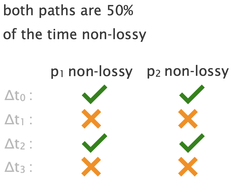

We also write equations for the performance of:

• “path pairs” which refer to two paths
• “path sets” which refer to a set of one or more paths

During a time interval,

• a path pair is “non-lossy” iff both of its paths are non-lossy
• a path set is “non-lossy” iff all of its paths are non-lossy

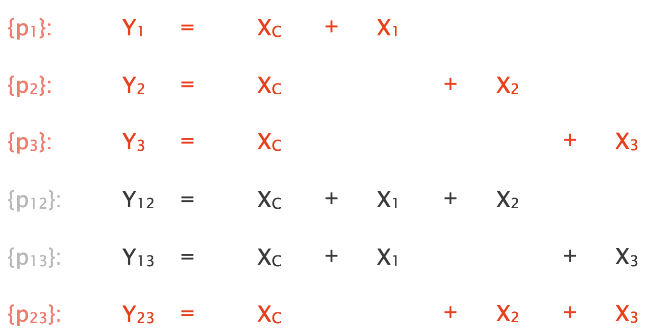
Revised: We build a system of equations by writing equations for the performance of pathsets

Here, additionally to paths, there is only path pair {p12} and we can write the following equation for it: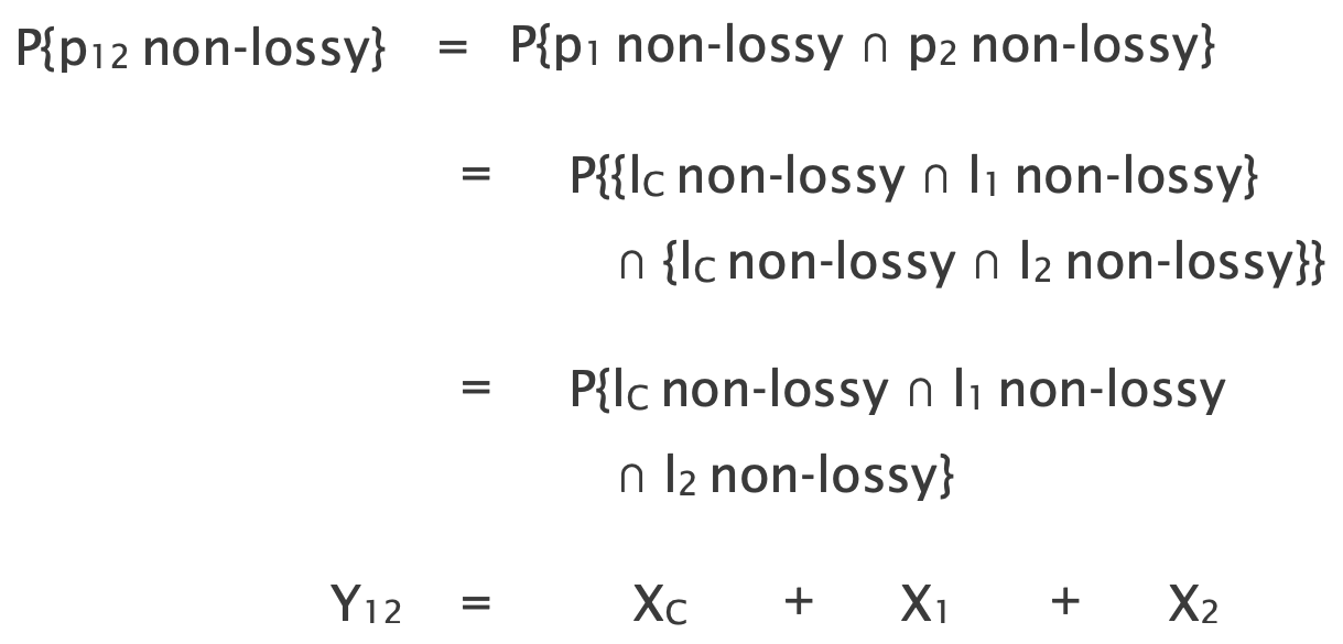

We estimate the probability of a path pair being non-lossy as the fraction of time intervals where both paths are non-lossy.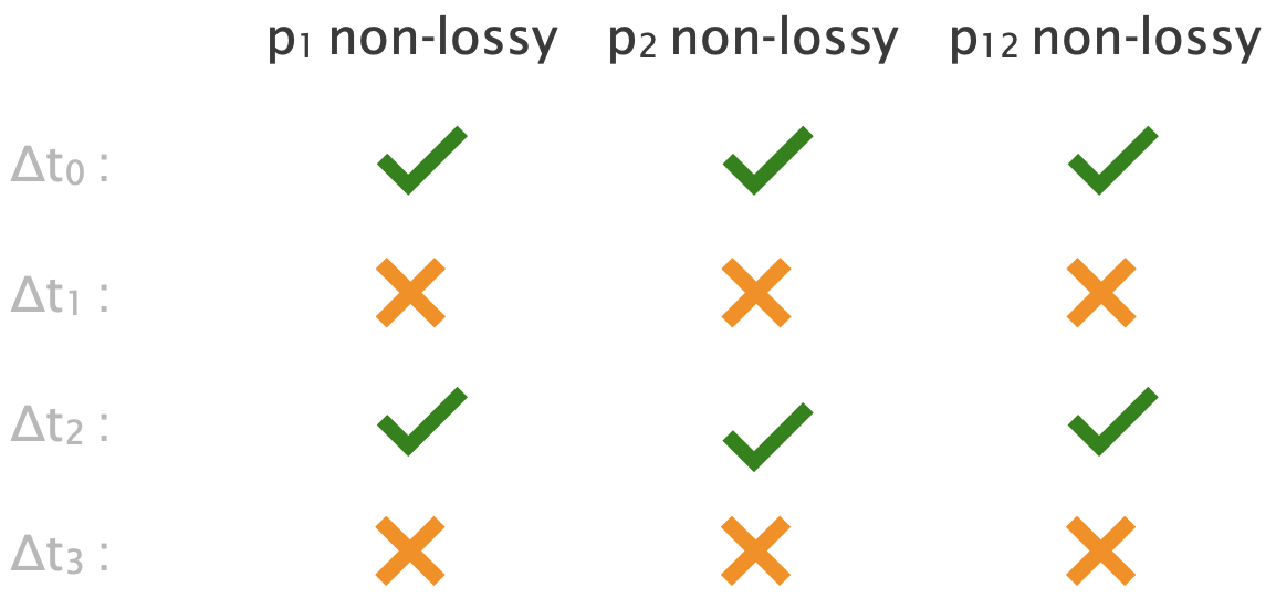

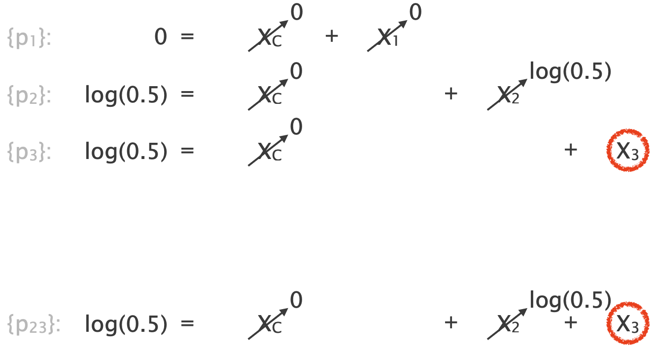
\[P(p_1\text{ non-lossy}) = 0.5\rightarrow Y_1=\log(0.5)\] \[P(p_2 \text{ non-lossy}) = 0.5\rightarrow Y_2=\log(0.5)\] \[P(p_{12} \text{ non-lossy}) = 0.5\rightarrow Y_{12}=\log(0.5)\]

This system of equations is full-rank so solving it yields a unique solution.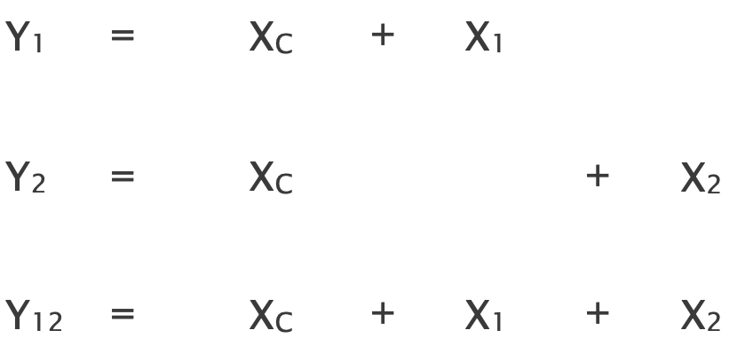

Since $X_1 = X_2= 0$ and $X_C = \log(0.5) < 0$, we correctly infer that $l_C$ is the lossy link

Assumptions

This system of equations relies on several assumptions

Assumption	Description
Stationarity	the loss behavior of a link is the same over time; we use a single variable to capture whether a link is lossy
Neutrality	the loss behavior of a link is the same for all paths crossing it for each link; we used the same variable across all equations
Stability	the paths remain unchanged over time; we use a single equation for each path
Independence	a link is lossy independently from other links; multiplied per-link probabilities to obtain the path probability
Separability	a path is non-lossy iff all of its links are non-lossy; on top of the path loss threshold, lossy links must be “severely” lossy

Given those assumptions and a full-rank system of equations, this tomography technique infers all lossy links. Consider the same network as before, but now not only $l_C$ but also $l_1$ is lossy w.p. $0.5$.

We can write the same equations as before and plug in the new path performance estimates: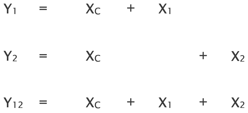

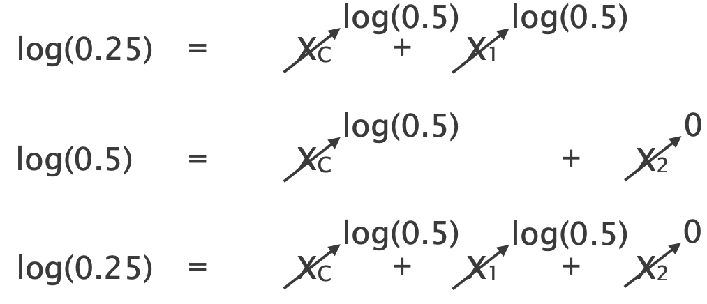
Since $X_2 = 0$ and $X_1 = X_C = \log(0.5) < 0$, we correctly infer that both links $l_1$ and $l_C$ are lossy.

In this slightly different network, there is no full-rank system as the performance of lC1 can always be attributed to lC2 and vice versa.

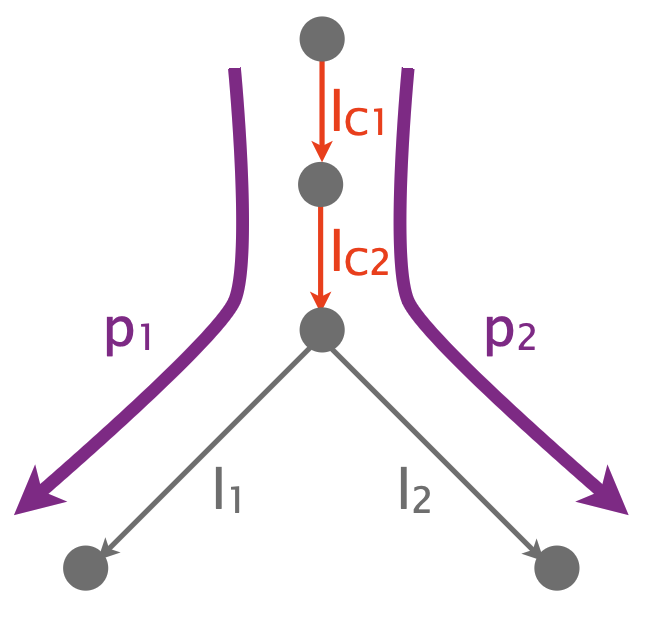
Sufficient conditions for having a full-rank system of equations:

1. We include in the system an equation for each path set (incl. individual paths)
2. Every two links are distinguishable: they are traversed by different sets of paths

In the initial network, we could build a full-rank system because any two links are traversed by different sets of paths: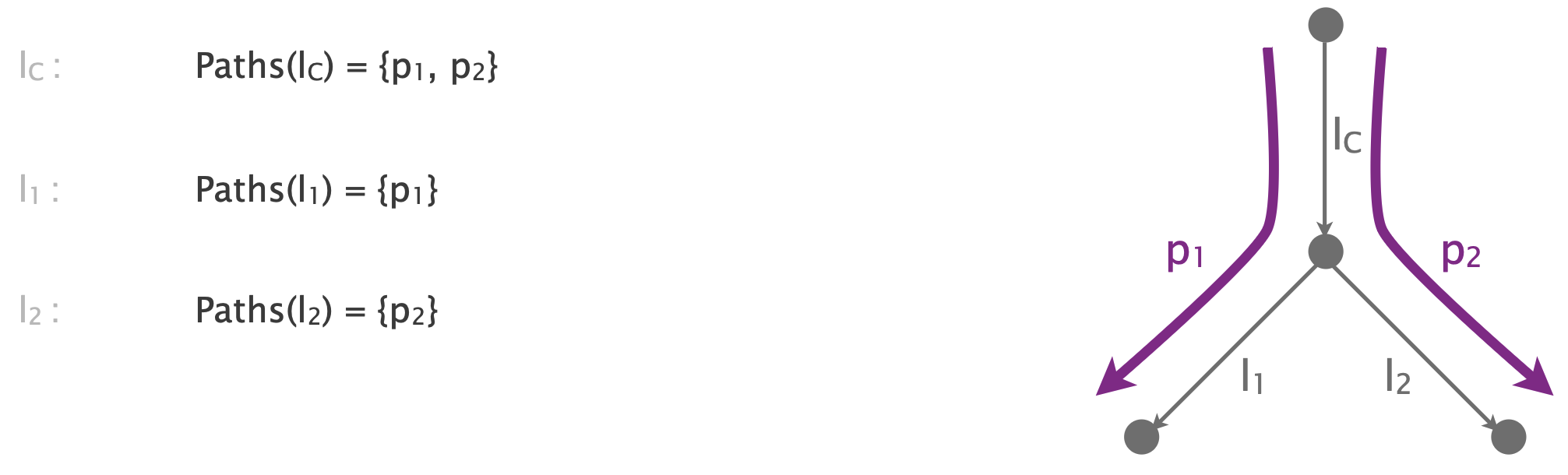

Link Neutrality

Consider another network with 4 links and 3 paths: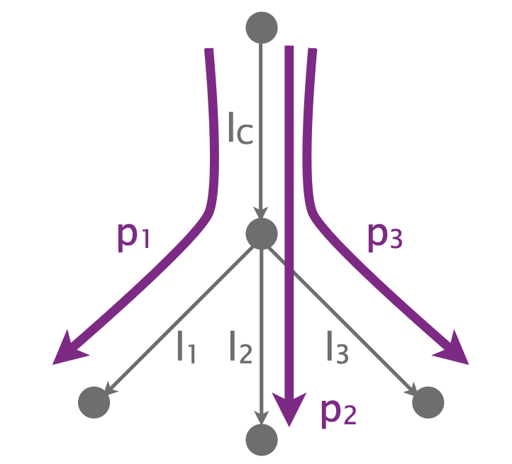

This is a non-neutral network: all links are always non-lossy except $l_C$, which is non-neutral and lossy only for p2/p3 traffic w.p. $0.5$.

An alternative way to think about this network is to use its neutral-equivalent network, where all links are neutral. 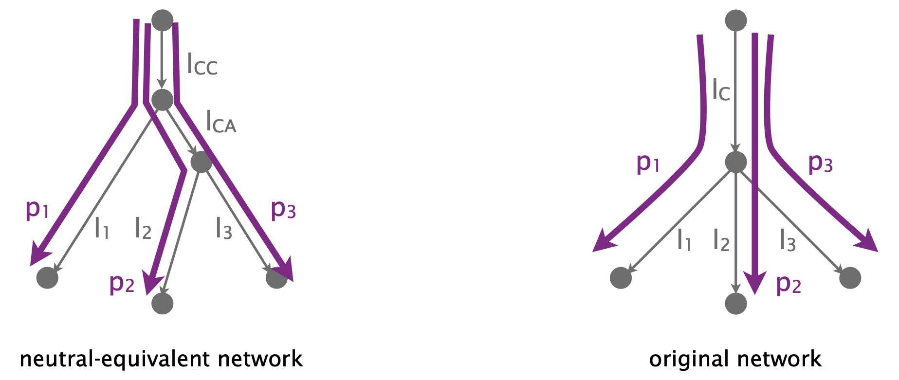In the neutral-equivalent network, the non-neutral link lC maps to two links:

• one for the common behavior (lCC)
• and one for the worse effect of lC on p2/p3 (lCA)

Here we are showing a snapshot of the network, during which lC is non-lossy for p1 but lossy for p2/p3 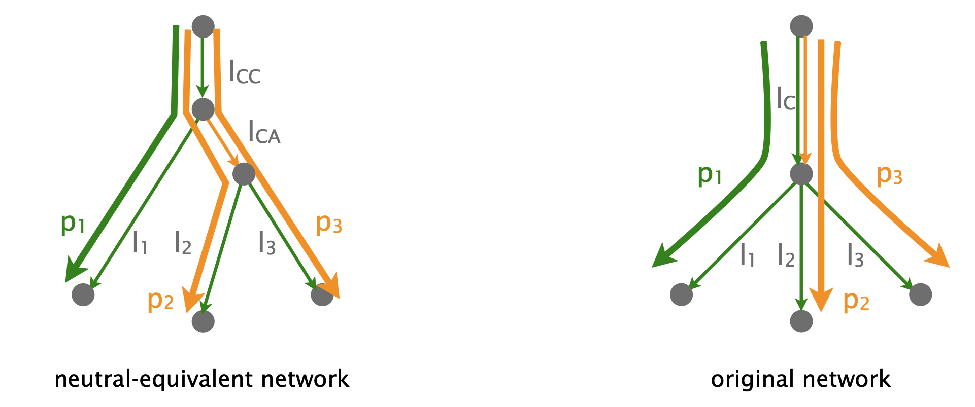In the neutral-equivalent network, lCC is not lossy but lCA is.

How do we identify that a certain link is non-neutral from the topology and path measurements?

The key insight is that wrongly assuming neutral links can lead to an unsolvable system.

• If we use a different variable to capture different link performance, then any system of equations we build is solvable.
• If we build an unsolvable system of equations, then we used the same variable for different link performance
  • $\rightarrow$ we wrongly assumed as neutral a non-neutral link

The key idea is to assume neutral links and build an unsolvable system that reveals that at least one link is non-neutral.

Our best chance is to write an equation for each path set using more info constrains more the system’s solutions. Still, we cannot always build an unsolvable system if a link’s worse effect on a path can be attributed to another link.

To identify that a certain link $λ$ is non-neutral, we carefully build the system of equations.

We write equations only for all path pairs that share only $λ$ and all their individual paths by mapping $λ$ to a single variable and for each path, all other links to a new variable

Intuitively,

• only λ assumed neutral => if unsolvable system, only this assumption can be wrong
• different path pairs may yield different solutions for λ => unsolvable system

Example

The path pairs that share only $λ = l_C$ are {p1, p2}, {p1, p3}, {p2, p3}, so $\Pi_λ = ((p1), (p2), (p3), (p1, p2), (p1, p3), (p2, p3))$

We build the following system for $\Pi_λ$: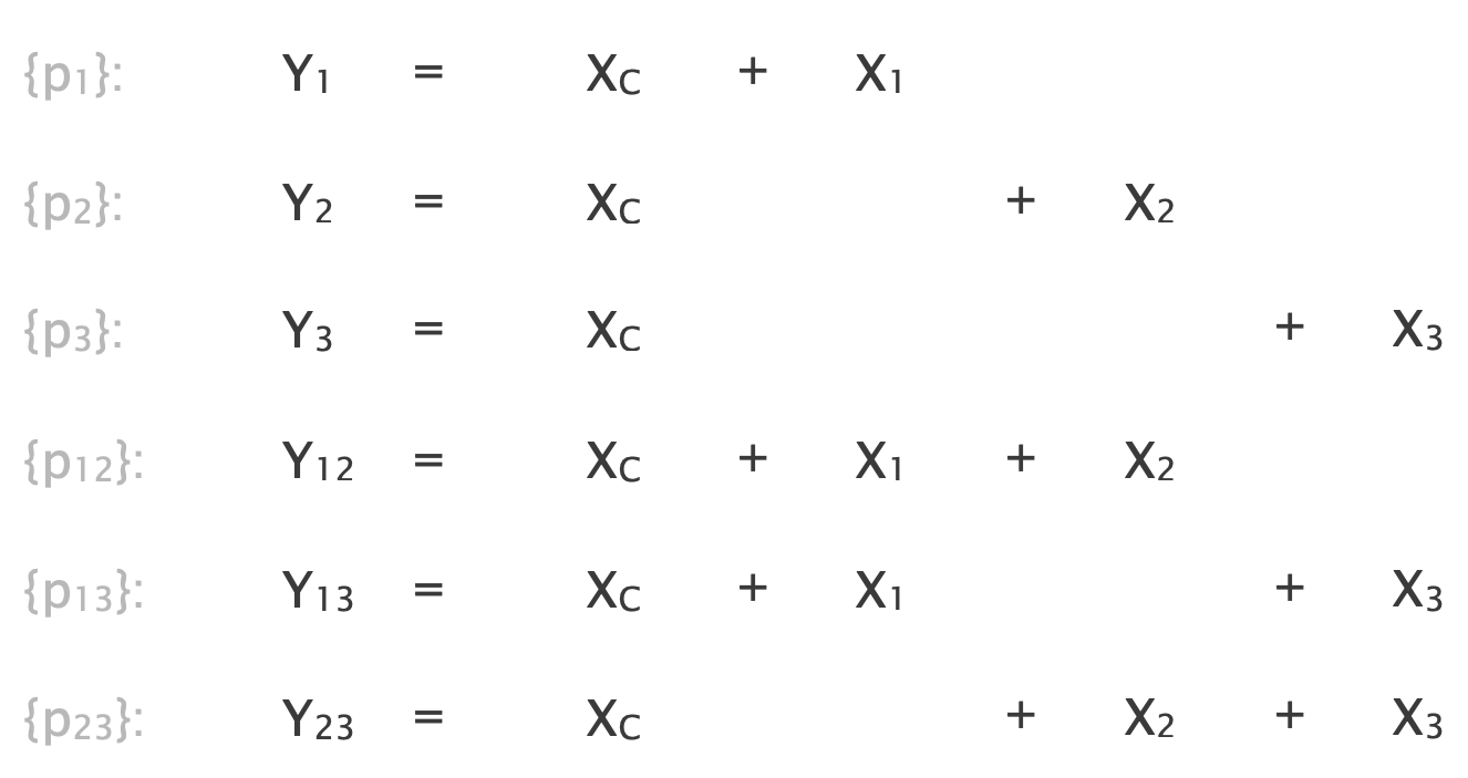

The following sub-system is unsolvable, hence the overall system as well

Since the system is unsolvable, we correctly identify that lC is non-neutral.

1. Probability of a link being non-lossy
2. Link neutrality

Tomography exploits correlations in end-to-end measurements to infer the performance of individual links