Hierarchical routing

Scaling networks

A scalable network is a network which supports a growing number of nodes, routes and destinations. To build it, we need control and data plane scalability.

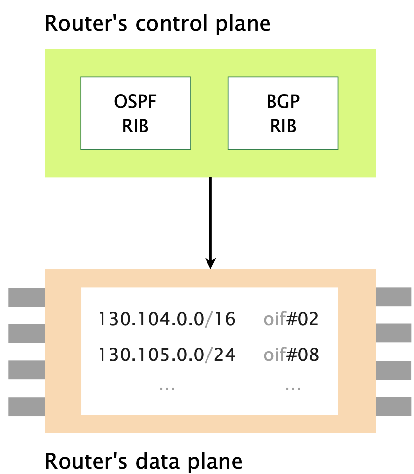
The control plane:

• maintains all the routes learned in Routing Information Bases (RIBs)
• computes the best route, for each destination prefix
• downloads the best route in the forwarding plane

The data plane:

• maintains the best routes in a Forwarding Information Base (FIB)
• forwards packets by performing longest-prefix match in the FIB

We’ll explore 2 complementary scaling techniques, both relying on hierarchy

1. hierarchical routing: how to optimize routes propagation

   Helps with scaling of number of routers, routes and prefixes

2. prefix aggregation and filtering: how to reduce the number of forwarding entries

   Only helps with scaling of prefixes

Inter-domain routing

eBGP and iBGP

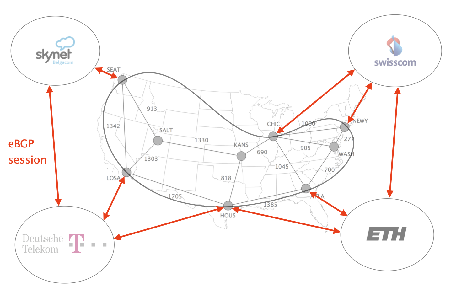
External BGP (eBGP) sessions connect border routers in different ASes.

Using eBGP sessions, border routers learn routes to external destinations.

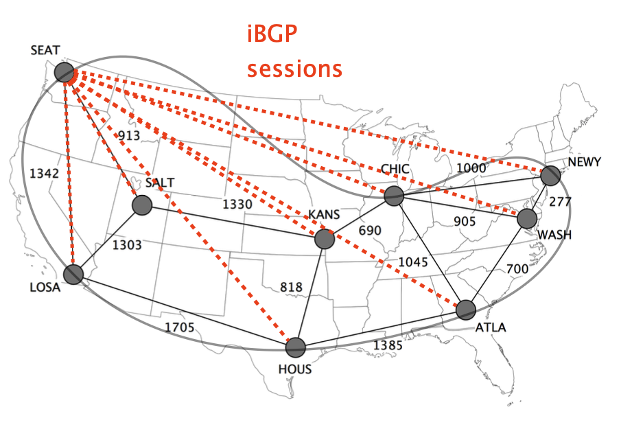
Internal BGP (iBGP) sessions connect the BGP routers within the AS.

Using iBGP sessions, internal BGP routers learn both externally-learned and internally-advertised routes

Given a set of {i,e}-BGP-learned routes, each BGP router elects one best route for each prefix.

BGP is often referred to as a “single path protocol”, and it picks the best route based on a set of rules.

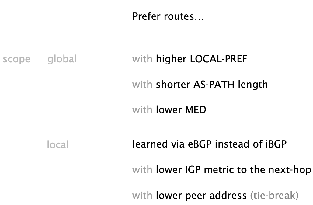
iBGP routers rely on the IGP (Internal Gateway Protocol) to figure out how to reach the egress next-hop. They also rely on the IGP cost to select their best route.

This process is also known as a recursive next-hop resolution.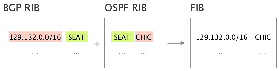

Inter-domain routing in a nutshell

Protocol	Purpose
eBGP	Learn and advertise routes from and to neighboring ASes
iBGP	disseminate internal and external routes withing the AS
IGP	Compute the shortest paths within the AS, identify closest egress point

iBGP routers do not redistribute their best iBGP-learned routes to other iBGP routers. This demands a iBGP full mesh, where, with $n$ iBGP routers, you need $\frac {n(n-1)} 2$ iBGP sessions. However, maintaining an iBGP full-mesh does not scale:

Property	Issue
state	Maintaining (too) many TCP connections, storing (too) many BGP routes per prefix
bandwidth	Sending every BGP update to every other router
management	Reconfiguring every router anytime one adds or remove one router

Route reflection

BGP route reflection alleviates the need for a full mesh by relaxing the iBGP propagation rules. It allows specific iBGP routers (known as route reflectors) to redistribute their best route.

• A route reflector establishes normal iBGP sessions identical to the ones used by default.
• These sessions are split between client and peers, identified by configuration.
• Reflection happens conditionally on the session type, very much like provider, peer and customers.

Route reflection enables to build a hierarchical iBGP propagation graph.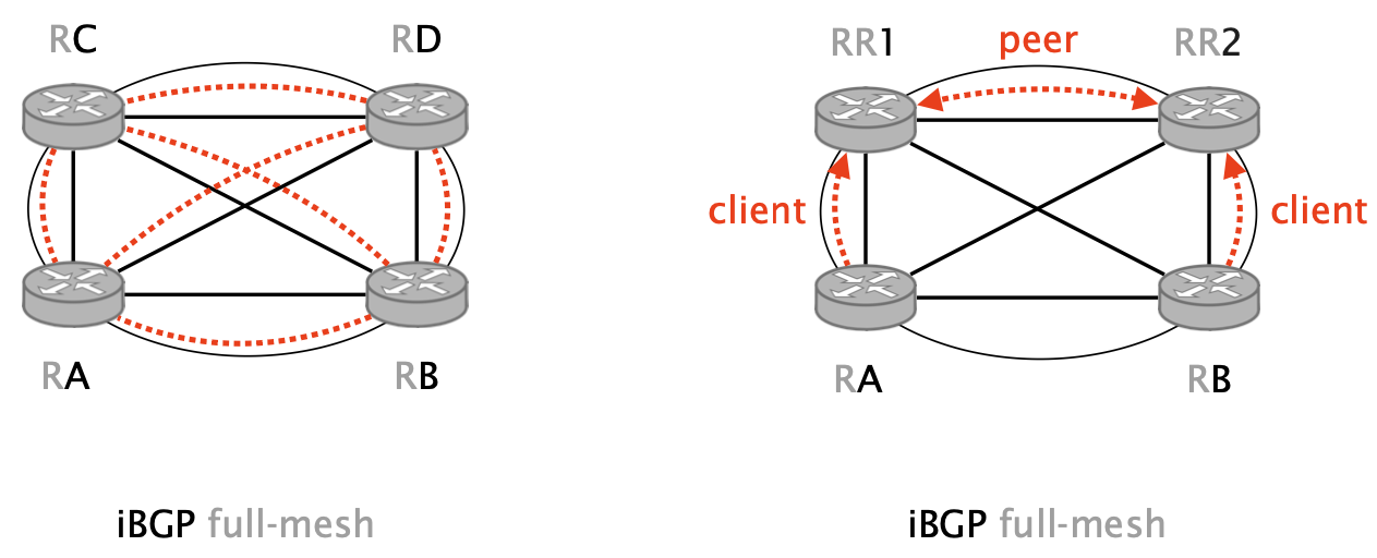

If the best route is learned from a peer, it is reflected to all clients. Otherwise, if it’s learned from a client or it is external, it is reflected to everyone (clients + peers) - like normal iBGP.

Trade-offs

Route reflection helps scaling but comes at the cost of:

• reduced route diversity
  • part of the traffic will be following suboptimal paths.
    • Reflector’s clients only learn a subset of the routes the ones selected by their route reflectors
    • This can lead to different routes being selected with respect to the choices made in a full-mesh
    • This is especially so if RR sees different IGP distances than its clients
• possible routing and forwarding anomalies
  • such as permanent oscillation, non determinism for routing
  • such as forwarding loops for forwarding

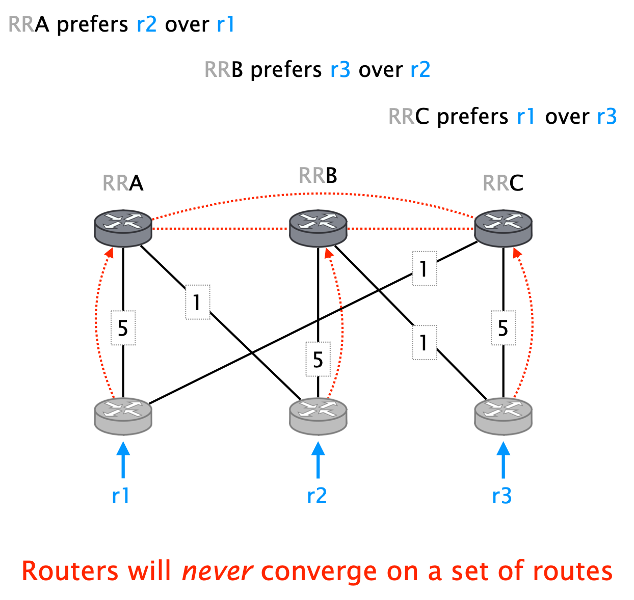
Unfortunately, deciding if an iBGP configuration is correct is NP-hard. There exist design practices to avoid problems:

• Ensure route reflector prefer client routes over peer, to prevent cycles from forming.
• Ensure BGP messages traverse the same path as data, to prevent forwarding deflections.
• Ensure route reflector is close to clients, to prevent inconsistent decisions.

Route reflector hierarchy

RRs can be “stacked” hierarchically, meaning a RR can have other RRs as clients. RRs are identified using a configurable cluster-ID:

• Internal routers get grouped into clusters
  • each AS can have one or more clusters
• Each cluster contains one or more Route Reflectors (RRs)
  • clusters are identified with a Cluster-ID
• RRs re-advertise internal routes within their clusters to all their clients

---

Intra-domain routing

In link-state routing, routers build a precise network map by flooding their local view to every other router.

• Each router keeps track of its incident links and costs as well as whether they are up or down.
• Each router broadcasts its own links’ states to give every router a complete view of the graph.
• Each router runs Dijkstra on the corresponding graph to compute their shortest-paths and forwarding tables.

The overhead of link-state protocols depends mostly on the network size. The larger the topology, the more it takes for routers to:

bandwidth	1. flood the link-state advertisements
memory	2. store the link-state database
processing power	2. compute the shortest paths

Improving scalability

There are two common strategies to improve the scalability of link-state protocols:

1. reduce Dijkstra’s shortest-path algorithm overhead
   1. optimizing its data structures
   2. reusing intermediate results, making the algorithm incremental
   3. running it less frequently by pacing computations using timers
2. introduce a hierarchy

incremental Shortest Path First

iSPF minimizes recomputation by analyzing the impact of topology changes.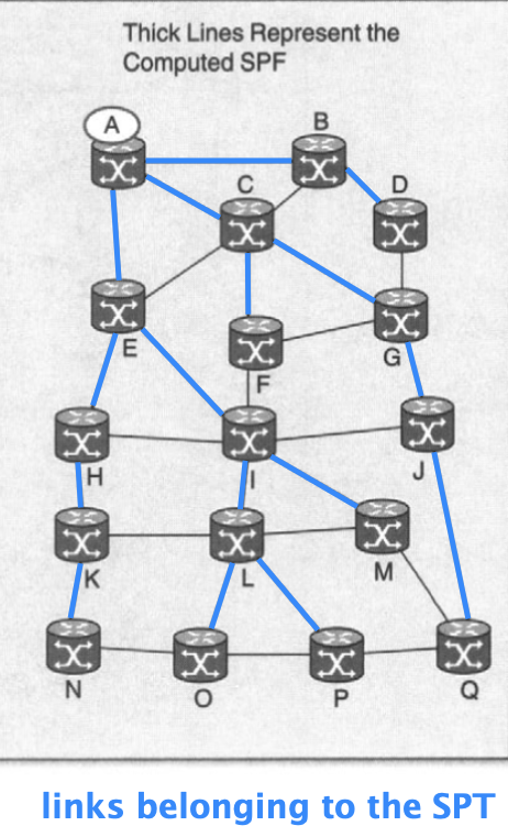

1. If the topology change only involves a new leaf or a link failure which does not belong to the previous shortest-path tree,

   • then the previous SPT is still correct, so iSPF does not need to recompute anything.

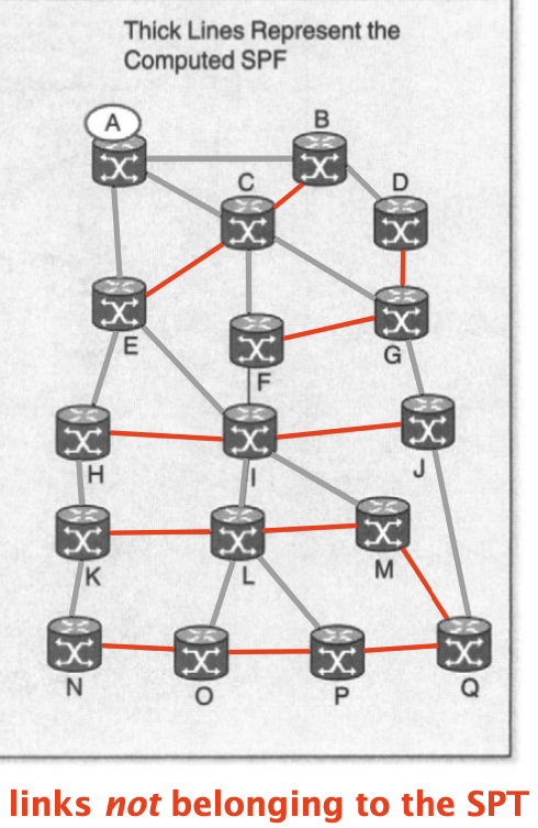
   • A red link failing will not affect the SPT computed by A because the failure of any of these links will never make a path better. Thus, A can skip the re-computation upon learning any such failure

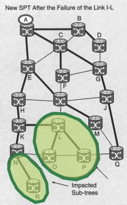
2. If the topology change only involves links that belong to the previous shortest-path tree,
   • then the previous SPT is not entirely correct anymore, but parts of it might still be. iSPF identifies the set of nodes impacted and restarts the computation from there.

A should only recompute subsets of its SPF tree. The failure of (I,L) only impacts the subtree rooted at L. The appearance of (N,R) only impacts the subtree rooted at N

The iSPF algorithm considers 2 main cases:

1. a link cost increase
2. a link cost decrease

iSPF Case 1

The link $L_{ij}$ sees its cost increase.

if Lij not in SPT:
    pass

else:
    Update distance FOR ALL nodes in the j-rooted subtree

    FOR EACH node k in the j-rooted subtree:
        check k's neighbors which are NOT in the tree for shorter paths

iSPF Case 2

The link $L_{ij}$ sees its cost decrease .

if Lij in SPT:
  Update distances for all nodes in the j-rooted subtree

  For each node k not in subtree:
    if k is a subtree neighbor:
      Check if shorter path available via the subtree

    else:
      delta = d(i) + cost(Lij) - d(j)
      
      if delta > 0: pass
      else:
        Lij is in the SPT. GOTO top.

Failure and recovery

iSPF also generalizes to node failure and recovery:

• Upon failure of node j:
  • Reattach nodes in the j-rooted subtree to the SPT by increasing the distance of each j-adjacent link to infinity.
• Upon recovery of node j:
  • Compute the shortest path to j by attaching it to its closest neighbor.
  • Check if shorter path available for all nodes whose distance from the source is greater than d_j

iSPF Gains

The gains of using iSPF heavily depend on where the topological changes are:

• iSPF gains tend to be substantial for faraway changes
  • as the impacted subtree tends to be small
• iSPF gains diminish as the change get closer to the source
  • as the impacted subtree tends to be large
• In (hopefully) few cases, iSPF gains can be negative
  • meaning that running iSPF is slower than a normal SPF

Introducing hierarchy

Hierarchical IGPs split the network into regions such that each region only knows topological details about itself.

One central area connects other peripheral areas, known as backbone and non-backbone areas respectively. Each area maintains its own link-state database. Area border router (ABR) only propagates path distances across: routers only know the cost to reach other areas’ destinations.

Areas alone only help so much: one advertisement per destination, still; even a single link failure may change multiple path costs.

For better scalability, ABR also need to summarize:

• The idea is to have one LSA for multiple prefixes, by having ABRs advertise less-specific prefixes.
• Each area relies upon unique, aggregatable addresses (it must be considered at design time).
• ABRs advertise summary prefixes across areas using as cost the maximum cost used to reach any sub-prefixes.

Summarization helps with scalability, but comes at a cost. While it reduces the size of the LSDB and confines changes to smaller regions, it also does lead to suboptimal routing and it’s more complex to operate.