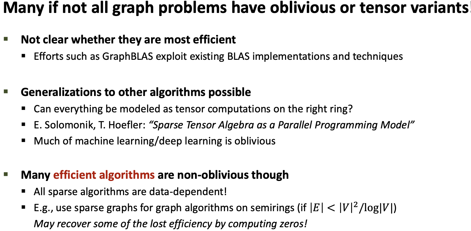
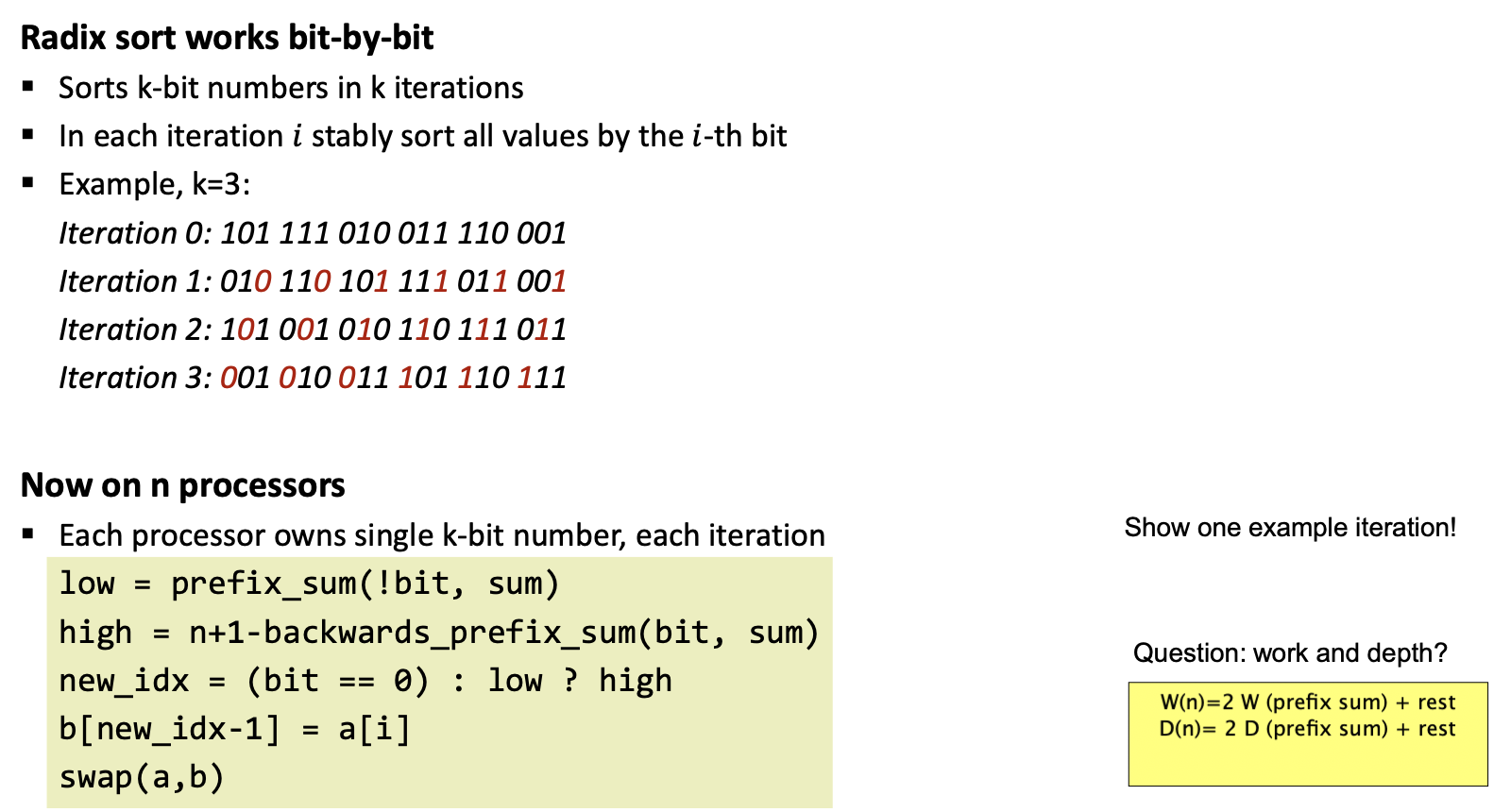
Oblivious Algorithms

Primer for Parallel Algorithms

The execution of programs can be described with Execution DAGs (EDAG)

• Each vertex is a basic calculation, and each edge is a dependency (value flowing)
• Work $W$ – number of operations performed when executing the algorithm
  • = sequential running time for $P=1$
• Depth D – minimal number of operations for any parallel execution
  • = parallel running time for $P=\infty$
  • Depth is also the longest path in the EDAG

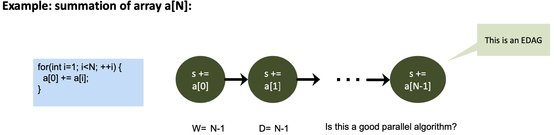
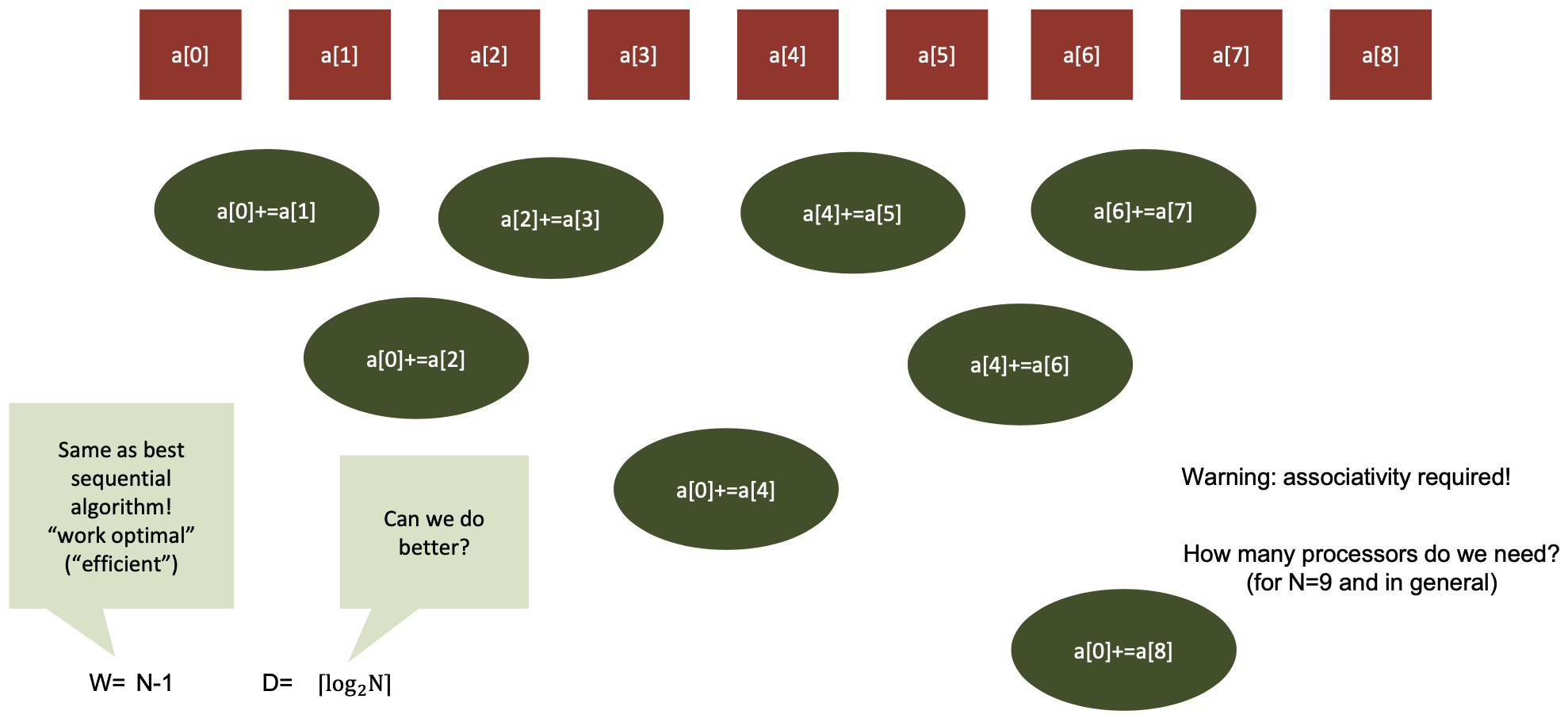
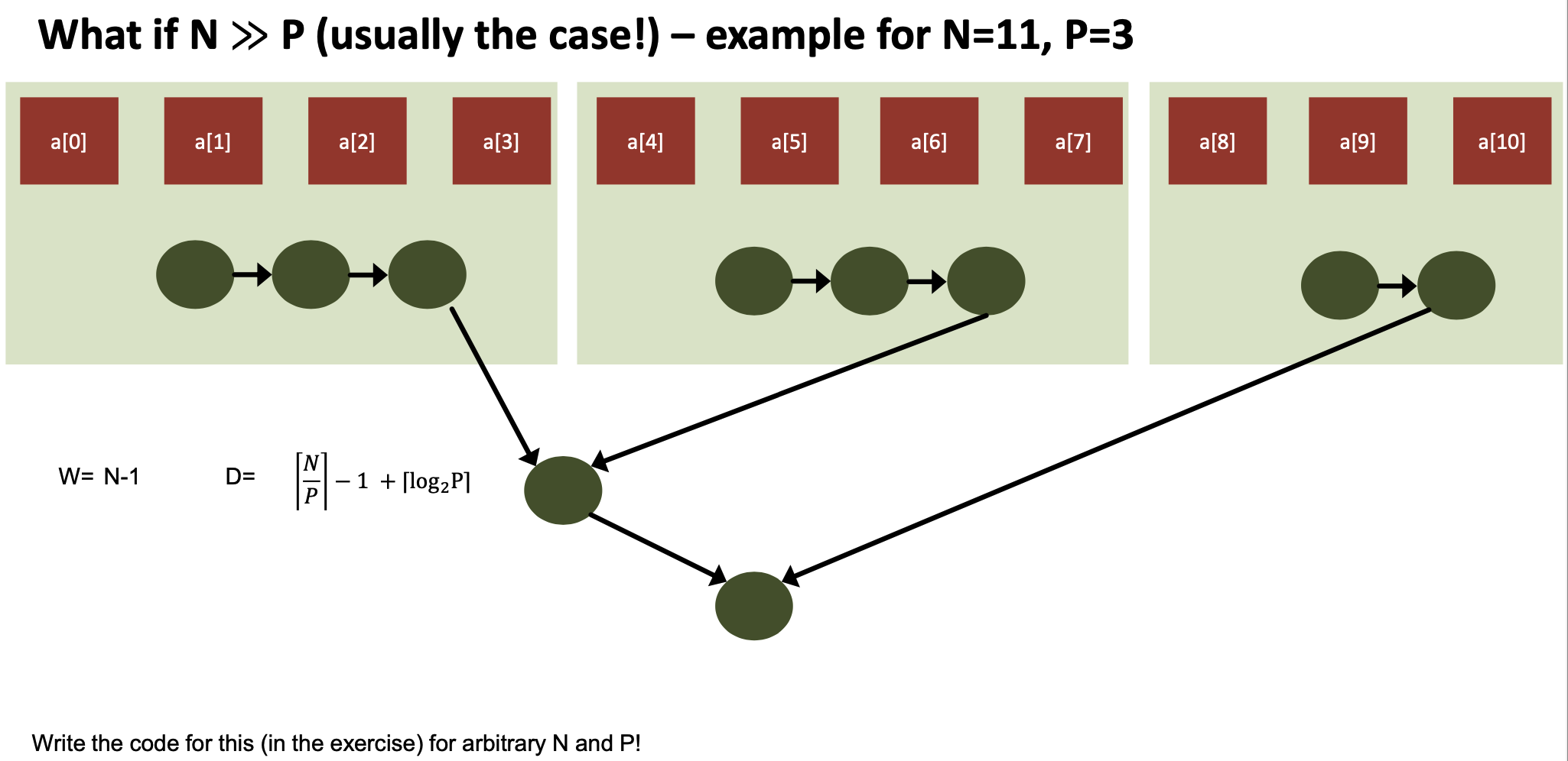
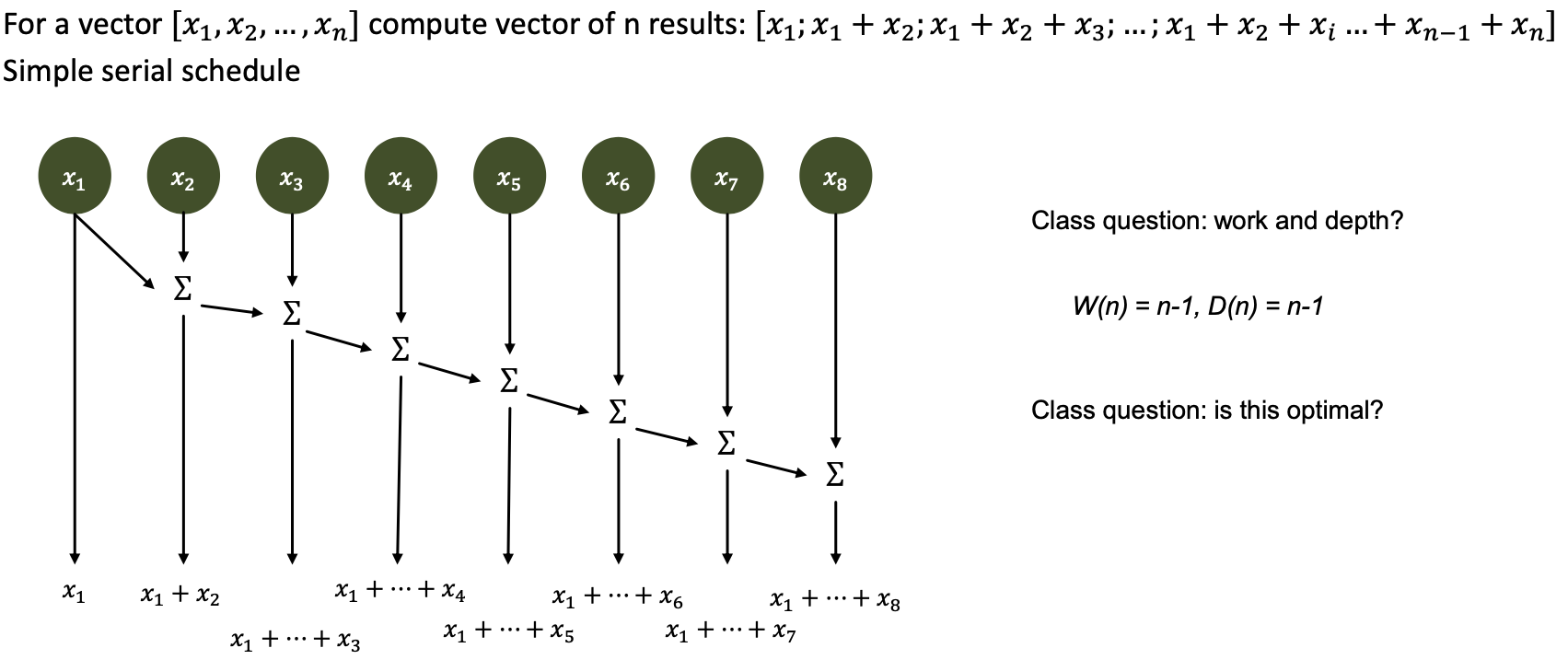
Parallel Summation (“Reduction”) – example for N=9

Work/Depth in Practice – Oblivious Algorithms

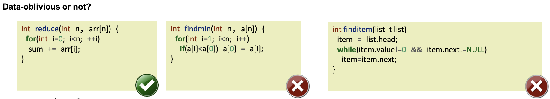
An algorithm is data-oblivious if, for each problem size, the sequence of instructions executed, the set of memory locations read, and the set of memory locations written by each executed instruction are determined by the input size and are independent of the values of the other inputs

Operation	Data Oblivious?
Quicksort?	No
Prefix sum on an array?	Yes
Dense matrix multiplication?	Yes
Sparse matrix vector product?	No
Dense matrix vector product?	Yes
Queue-based breadth-first search?	No

Can an algorithm decide whether a program is oblivious or not?

Answer: no, proof similar to decision problem whether a program always outputs zero or not

Structural obliviousness as stronger property

A program is structurally-oblivious if any value used in a conditional branch, and any value used to compute indices or pointers is structurally-dependent only on the input variable(s) that contain the problem size, but not on any other input

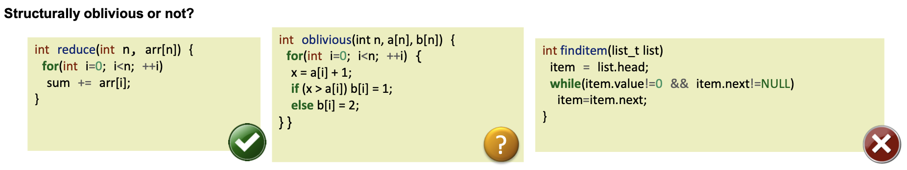
Structurally oblivious programs are also data oblivious!

• Can be programmatically (statically) decided
• Sufficient for practical use

The middle example is not structurally oblivious but data oblivious

• First branch is always taken (assuming no overflow) but static dependency analysis is conservative

Why obliviousness?

We can easily reason about oblivious algorithms

• Execution DAG can be constructed “statically”
  • we can even build circuits for fixed $N$ (HW acceleration!)
• We have done this intuitively, but we never looked at BFS for example

Simple example: parallel summation

• Question: what is $W(n)$ and $D(n)$ of sequential summation?

\[W(n)=D(n)=n-1\]

---

• Question: is this optimal? How would you define optimality?
  • Separate for $W$ and $D$! Typically try to achieve both optimally!

---

• Question: what is W(n) and D(n) of the optimal parallel summation?

\[W(n)=n-1\] \[D(n)=⌈\log_2 n⌉\]

• Are both $W$ and $D$ optimal?
  • Yes!

---

Scan

Algorithm

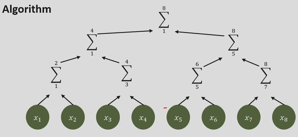
After going up, we have the sums of all the powers of 2. We’re missing $n-\log n$ elements. We need to go down to get the final result.

• work? (hint: after the way up, all powers of two are done, all others require another operation each)
  • $W (n) = 2n − \log_2 n − 1$
• depth? (needs to go up and down the tree)
  • $D (n) = 2 \log_2 n − 1$

Invest more work to reduce depth and thus get better parallelism!

Dissemination/recursive doubling

Recursive to get to $𝑾 = 𝑶 (𝒏)$ and $𝑫 = 𝑶(\log (𝒏))$! (Assume $𝒏 = 𝟐𝒌$ for simplicity!)

Idea: don’t reuse intermediate values, recompute them!

• Sounds “optimal”, doesn’t it? Well, let’s look at the constants!

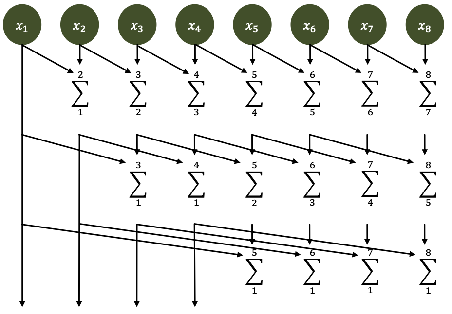
• Work? (hint: count number of omitted ops)
  • $W (n) = n \log_2 n − n + 1$
    • $\log_2 n$ rounds, maximum $n$ ops per round, $n − 1$ ops omitted per round (the tree on the left has depth $\log_2 n$, thus $n$ elements)
• Depth?
  • $D (n) = \log_2 n$

We now have a depth-optimal algorithm, but it’s not work-optimal!

Is there a depth- and work-optimal algorithm?

The answer is, surprisingly, no.

• We know, for parallel prefix: $W + D ≥ 2n − 2$

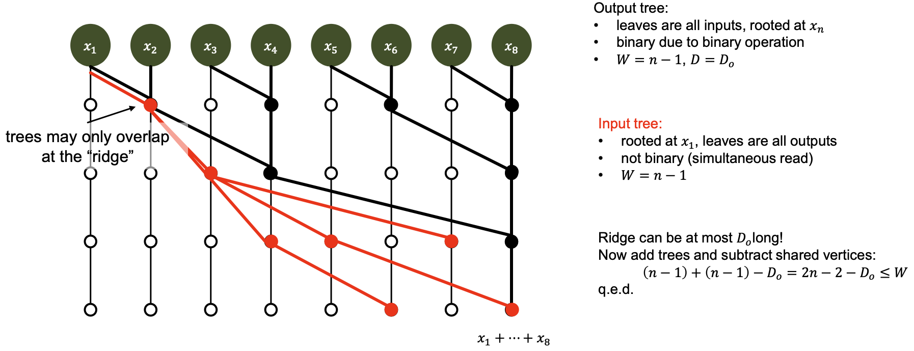
Work-Depth Tradeoffs and deficiency

Deficiency

“The deficiency of a prefix circuit c is defined as $def (c) = W_c + D_c− (2n − 2)$

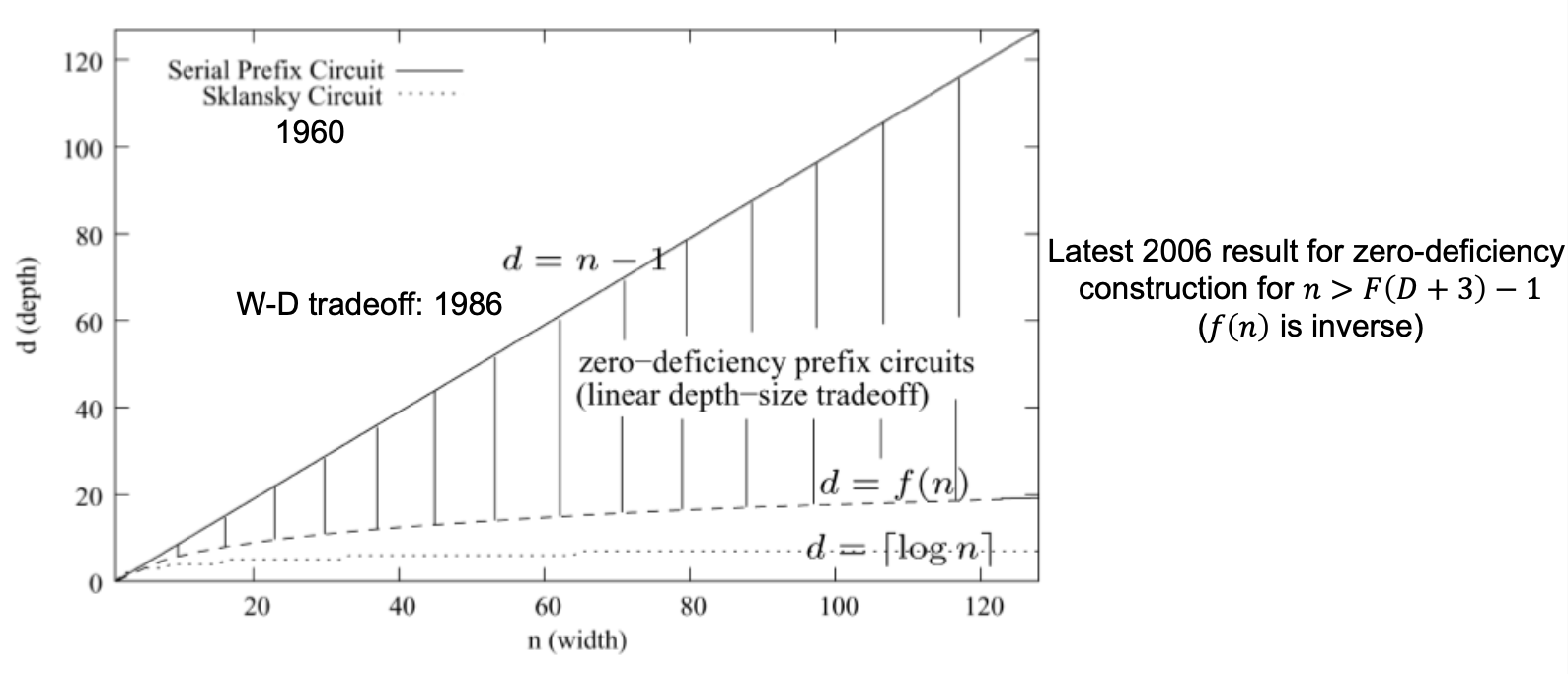
Work- and depth-optimal constructions

Work-optimal?

• Only sequential! Why?
• $W = n − 1$, thus $D = 2n − 2 − W = n − 1$ q.e.d.

Depth-optimal?

• Ladner and Fischer propose a construction for work-efficient circuits with minimal depth
  • $D = ⌈\log_2 n⌉, W ≤ 4n$
  • Simple set of recursive construction rules
  • Has an unbounded fan-out! May thus not be practical

Depth-optimal with bounded fan-out?

• Some constructions exist, interesting open problem

Why do we care about this prefix sum so much?

It’s the simplest problem to demonstrate and prove $W-D$ tradeoffs, and it’s one of the most important parallel primitives.

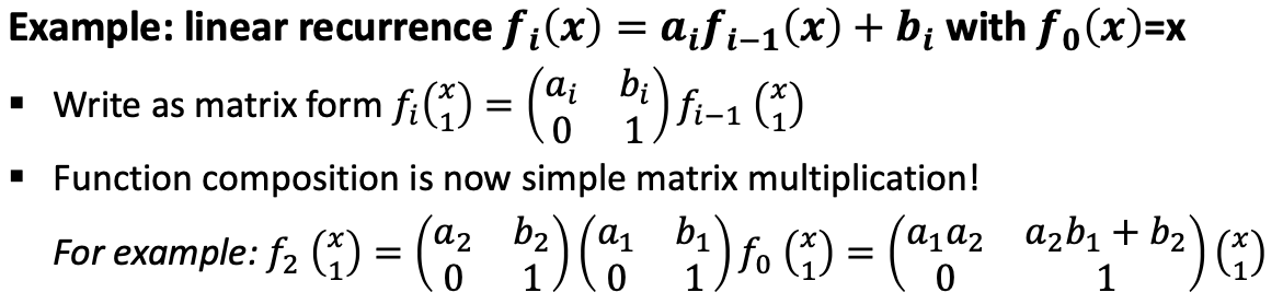
Prefix summation as function composition is extremely powerful!

With prefix summation many seemingly sequential problems can be parallelized.

Simple first example: binary adder – $s = a + 𝑏$ ($n$-bit numbers)

• Starting with single-bit (full) adder for bit i

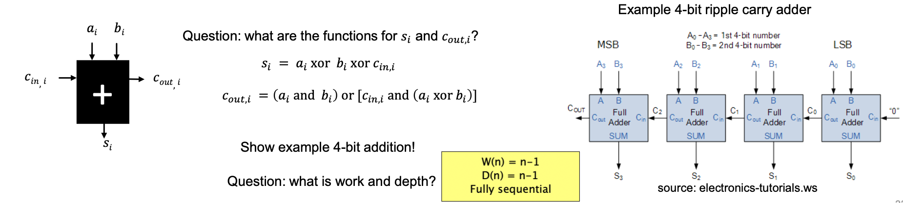
Seems very sequential, can this be parallelized?

We only want 𝒔!

• Requires $c_{in,1}, c_{in,2}, … , c_{in,n}$ though

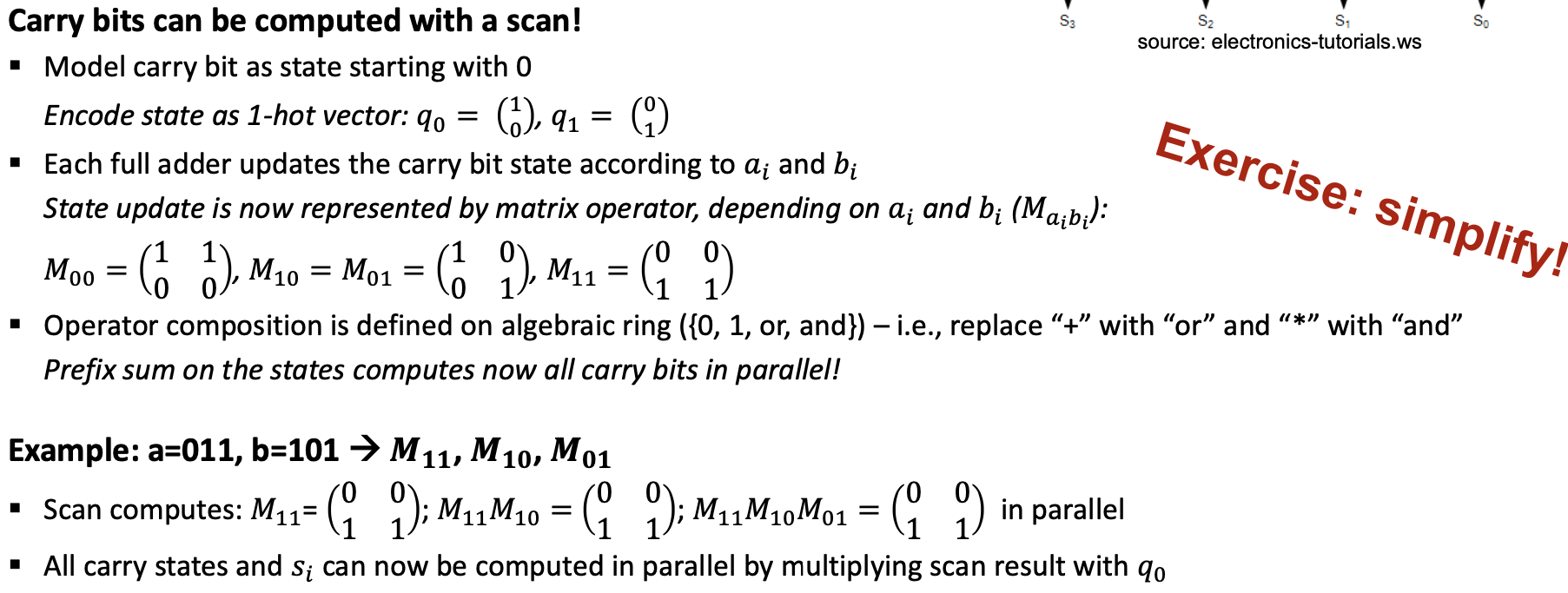
Prefix sums as magic bullet for other seemingly sequential algorithms

Any time a sequential chain can be modeled as function composition!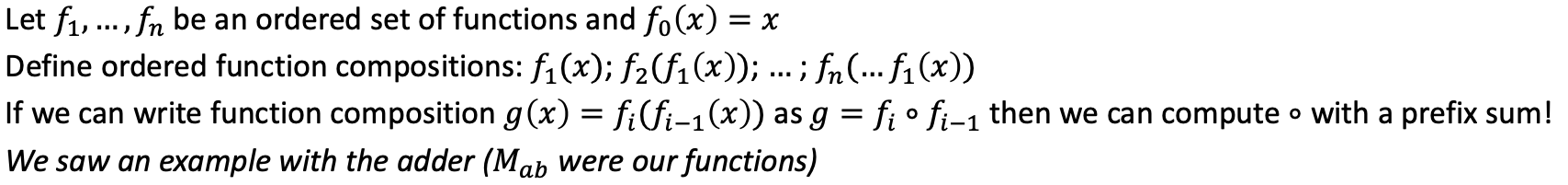

Another use for prefix sums: Parallel radix sort

Oblivious graph algorithms

Seems paradoxical but isn’t (may just not be most efficient)

• Use adjacency matrix representation of graph – “compute with zeros”

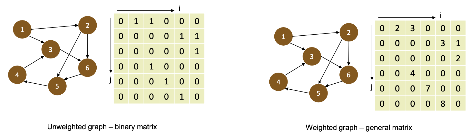
Algebraic semirings

A semiring is an algebraic structure that

• Has two binary operations called “addition” and “multiplication” on a set $S$
• Addition must be
  • associative $((a+b)+c = a+(b+c))$
  • and commutative $a+b=b+a$
  • and have an identity element
• Multiplication must be
  • associative
  • and have an identity element
• Multiplication distributes over addition $(a(b+c) = ab+a*c)$
  • →Multiplication by additive identity annihilates

Semirings are denoted by tuples $(S, +, *, \text{additive identity}, \text{multiplicative identity})$

Examples:

• Standard ring of rational numbers: $(ℝ, +, *, 0, 1)$
• Boolean semiring: $({0,1}, ∨, ∧, 0, 1)$
• Tropical semiring: $(ℝ ∪ {\infty}, min, +, \infty, 0)$
  • (also called min-plus semiring)

Oblivious shortest path search on $(ℝ ∪ {\infty}, \min, +, \infty, 0)$

Construct distance matrix from adjacency matrix by replacing all off-diagonal zeros with $\infty$

• Initialize distance vector $d_0$ of size $n$ to $\infty$ everywhere, but $0$ at start vertex.
  • e.g., $d_0 = (\infty, 0, \infty, \infty, \infty, \infty )^T$
  • Show evolution when multiplied!
• SSSP can be performed with $n+1$ matrix-vector multiplications!

Question: total work and depth?

• $W = O(n^3)$
• $D = O(n \log n)$

Question: Is this good? Optimal?

• Nope: Dijkstra $=O( E + V \log V )$

Oblivious connected components on $({0,1}, ∨, ∧, 0, 1)$

Question: How could we compute the transitive closure of a graph?

• Multiply the matrix $(A + I)$ $n$ times with itself in the Boolean semiring!
• Why?
  • Demonstrate that $(A + I)^2$ has 1s for each path of at most length $1$
  • By induction show that $(A + I)^ k$ has 1s for each path of at most length $k$

What is work and depth of transitive closure?

• Repeated squaring!
• $W = O(n^3\log n)$ $D = O(\log^2n)$
  • $\lceil \log_2 n\rceil$ multiplications (think $A^4 = {A^2}^2$ )

---

How to get to connected components from a transitive closure matrix?

• Each component needs unique label
• Create label matrix $𝐿_{ij} = j$ iff $(AI)^n_{ij}$ = 1 and $L_{ij} = \infty$ otherwise
• For each column (vertex) perform min-reduction to determine its component label!

Overall work and depth?

• $W = O(n^3\log n)$, $D = O(\log^2n)$