Distributed Networking

Bandwidth vs. Latency

Transfer time

\[T(s) = \alpha + \beta s\]

• $\alpha $ = startup time (latency)
• $\beta $ = cost per byte (bandwidth = $1/\beta $)

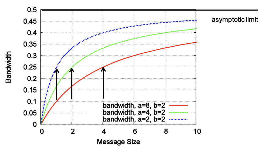
Effective bandwidth of a transfer:

• $E(s) = s / T(s)$

As $s$ increases, the effective bandwidth approaches $1/\beta $ asymptotically

• Convergence rate depends on α
• $s_{1/2} = \alpha /\beta $

Assuming no pipelining (new messages can only be issued from a process after all arrived)

• Two messages of size s between two processes cost $2(\alpha + s\beta )$
• Somewhat unrealistic (networks pipeline) but simple for now – we will lift this later!

$s_{1/2} = \alpha /\beta $ is often used to distinguish bandwidth- and latency-bound messages

• $s_{1/2} $ is in the order of kilobytes on real systems

Examples

Simplest linear broadcast

• One process has a data item to be distributed to all processes

Linearly broadcasting $s$ bytes among $P$ processes:

\[T (s) = (P − 1) ⋅ (\alpha + \beta s) = O(P)\]

k-ary Tree Broadcast

Origin process is the root of the tree, passes messages to $k$ neighbors which pass them on

• $k=2 \rightarrow$ binary tree

What is the broadcast time in the simple latency/bandwidth model?

• $T (s) ≈ \log_kP ⋅ k(\alpha + \beta s)$ (for fixed k)

What is the optimal $k$?

\[0 = \frac {k \ln P} {\ln k} \frac {d} {dk} = \frac {\ln P \ln k - \ln P} {\ln^2 k} \rightarrow k = e \approx 2.71\]

Independent of $P, \alpha, \beta, s$?

Faster Trees?

Can we broadcast faster than in a ternary tree?

• Yes, because each non-leaf processor is idle after sending three messages!
• Those processors could keep sending!
• Result is a k-nomial tree
• For $k=2$, it’s a binomial tree

What about the runtime?

• $T (s) ≈ \log_kP ⋅ k(\alpha + \beta s)=O(\log P)$

What is the optimal $k$ here?

• $T(s) \frac d {dk}$ is monotonically increasing for $k>1$, thus $k_{opt}=2$

Can we broadcast faster than in a k-nomial tree?

• $O(\log P)$ is asymptotically optimal for $s=1$
• But what about large $s$?

Very Large Message Broadcast

Extreme case (P small, s large): simple pipeline

• Split message into $P$ segments
• Send segments from $PE_i$ to $PE_{i+1}$
• What is the runtime? $T(s) = (P − 1)(\alpha + \frac s P \beta)$

Compare $2$-nomial tree with simple pipeline for $α=10, β=1, P=4, s=10^6$

• $2,000,020$ vs. $1,000,030$

Can we do better for given $α, β, P, s$?

• Yes, mix those algorithms – quite complex!

What is a simple lower bound on the broadcast time?

\[T_{BC} \geq\min(\lceil\log_2(P)\rceil\alpha,s\beta)\]

How close are the binomial tree for small messages and the pipeline for large messages (approximately)?

• Binary tree is a factor of $\log_2(P)$ slower in bandwidth
• Pipeline is a factor of $\frac P{\log_2(P)}$ slower in latency

What can we do for intermediate message sizes?

• Combine pipeline and tree → pipelined tree

What is the runtime of the pipelined binary tree algorithm?

\[T \approx (\frac s z \lceil \log_2 P\rceil-2)\cdot2\cdot(\alpha +z\beta)\]

What is the optimal $z$?

\[z_{opt}=\sqrt{\frac {\alpha s} {\beta(\lceil \log_2P \rceil-2)}}\]

Towards an Optimal Algorithm

What is the complexity of the pipelined tree with $z_{opt}$ for small $s$, large $P$ and for large $s$, constant $P$?

• Small messages, large $P$: $s=1; z=1$ $(s≤z)$, will give $O(\log P)$
• Large messages, constant $P$: assume $α, β, P$ constant, will give asymptotically $O(sβ)$

Asymptotically optimal for large P and s but bandwidth is off by a factor of 2! Why?

Intuition:

• In a binomial tree, all leaves ($P/2$) only receive data and never send
  • results in wasted bandwidth
• Send along two simultaneous binary trees where the leaves of one tree are inner nodes of the other
• Construction needs to avoid endpoint congestion

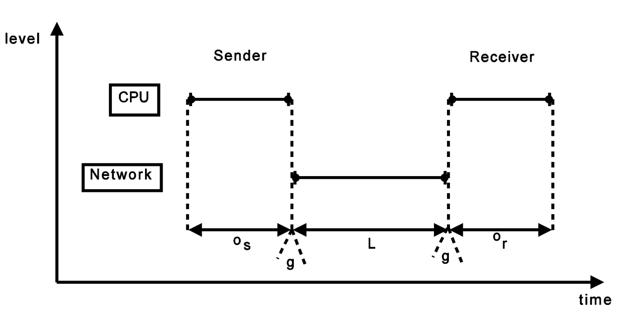
The LogP Model

Defined by 4 parameters:

• L: an upper bound on the latency, or delay, incurred in communicating a message containing a word (or small number of words) from its source module to its target module.
• o: the overhead, defined as the length of time that a processor is engaged in the transmission or reception of each message; during this time, the processor cannot perform other operations.
• g: the gap, defined as the minimum time interval between consecutive message transmissions or consecutive message receptions at a processor. The reciprocal of g corresponds to the available per-processor communication bandwidth.
• P: the number of processor/memory modules.

We assume unit time for local operations and call it a cycle.

Examples

Sending a single message	$T = 2o+L$
Ping-Pong Round-Trip	$T_{RTT} = 4o+2L$
Transmitting n messages	$T(n) = L+(n-1)\cdot\max(g, o) + 2o$

Simplifications

1. $o > g$ on some machines
   • $g$ can be ignored (eliminates max() terms)
   • be careful with multi-core!
2. Offloading networks might have very low $o$
   • Can be ignored (not yet but hopefully soon)
3. $L$ might be ignored for long message streams
   • If they are pipelined
4. Account $g$ also for the first message
   • Eliminates $-1$

Benefits over Latency/Bandwidth Model

Models pipelining

• $\frac L g$ messages can be “in flight”
• Captures state of the art (cf. TCP windows)

Models computation/communication overlap

• Asynchronous algorithms

Models endpoint congestion/overload

• Benefits balanced algorithms

Example: Broadcasts

What is the LogP running time for a linear broadcast of a single packet?

\[T_{lin} = L + (P-2) * \max(o,g) + 2o\]

---

Approximate the LogP runtime for a binary-tree broadcast of a single packet?

\[T_{bin} ≤ \log_2P * (L + \max(o,g) + 2o)\]

---

Approximate the LogP runtime for an k-ary-tree broadcast of a single packet?

\[T_{k-n} ≤ \log_kP * (L + (k-1)\max(o,g) + 2o)\]

---

Approximate the LogP runtime for a binomial tree broadcast of a single packet (assume $L> g$!)?

\[T_{bin} ≤ \log_2P * (L + 2o)\]

---

Approximate the LogP runtime for a k-nomial tree broadcast of a single packet?

\[T_{k-n} ≤ \log_kP * (L + (k-2)\max(o,g) + 2o)\]

---

What is the optimal $k$ (assume $o>g$)?

• Derive by $k$: $0 = o * \ln(k_{opt}) – L/k_{opt} + o$ (solve numerically)
  • For larger $L$, $k$ grows and for larger $o$, $k$ shrinks
• Models pipelining capability better than simple model!

---

Can we do better than $k_{opt}$-ary binomial broadcast?

• Problem: fixed $k$ in all stages might not be optimal
• We can construct a schedule for the optimal broadcast in practical settings

Optimal Broadcast

Broadcast to $P-1$ processes

• each process who received the value sends it on;
• each process receives exactly once.

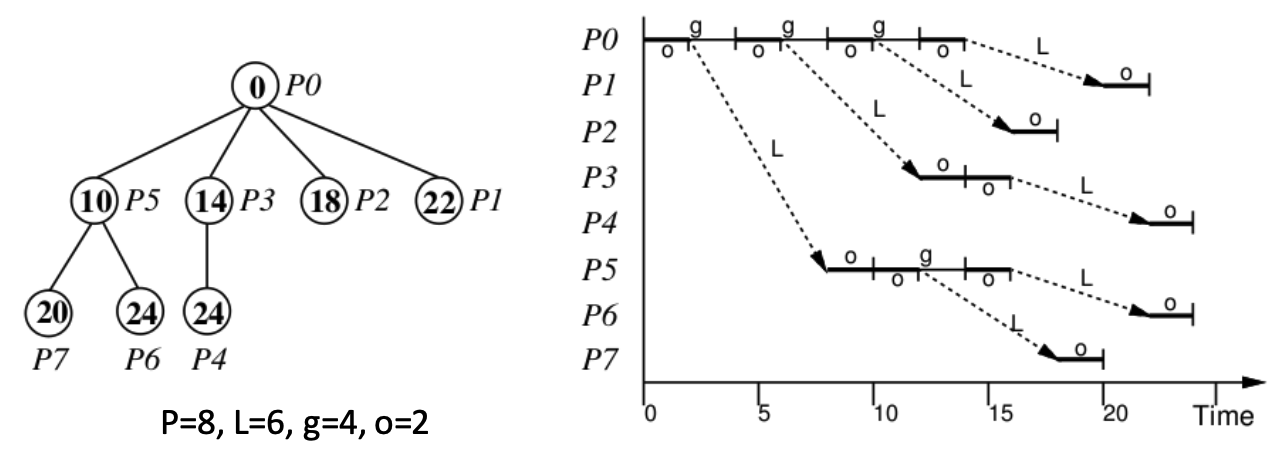
Optimal Broadcast Runtime

This determines the maximum number of PEs ($P(t)$) that can be reached in time $t$

• $P(t)$ can be computed with a generalized Fibonacci recurrence (assuming $o>g$):

\[P(t)=\begin{cases} 1: \quad \quad \quad \quad \quad \quad \quad \quad \quad \quad \, \,t<2o+L\\ P(t-o) + P(t-2o-L): t≥2o+L \end{cases}\]

• which can be bounded by

\[2^{\lfloor \frac {t}{L+2o} \rfloor} ≤P(t)≤2^{\lfloor \frac t o \rfloor}\]